1. Introduction

LeNet-5 was one of the earliest deep learning models, introduced in 1998 in the paper “Gradient-Based Learning Applied to Document Recognition” by Yann LeCun, Léon Bottou, Yoshua Bengio, and Patrick Haffner. Several of these authors went on to make major contributions to the field of deep learning.

From left: Yann LeCun, Leon Bottou, Yoshua Bengio, and Patrick Haffner

This article introduces the LeNet-5 CNN architecture as described in the original paper, walks through an implementation using TensorFlow 2.0, and finishes by using that implementation to classify images from the MNIST dataset.

What you’ll find in this article:

• An overview of the components that make up a convolutional neural network
• Definitions of terms commonly used in deep learning and machine learning
• A walkthrough of the LeNet-5 architecture as presented in the original paper
• An implementation of the network using TensorFlow and Keras

This article is written for deep learning and machine learning students of all levels. If you’re eager to get to the code, jump straight to the Implementation section.

2. Convolutional Neural Networks

Convolutional neural networks (CNNs) are the standard architecture for tasks involving images. Object detection, face detection, pose estimation, and many other computer vision tasks are usually solved with some variant of a CNN.

A handful of characteristics make CNNs particularly well suited to computer vision tasks. Before diving into LeNet-5, it’s worth introducing them:

• Local receptive fields
• Sub-sampling
• Weight sharing

The LeNet-5 architecture is made up of seven layers: three convolutional layers, two sub-sampling layers, and two fully connected layers.

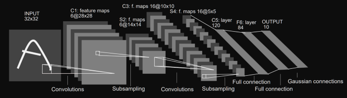
LeNet architecture

The diagram above shows the LeNet-5 architecture as illustrated in the original paper.

The first layer is the input layer, which isn’t generally counted as a true layer of the network since nothing is learned there. It’s built to accept 32x32 images. Since MNIST images are 28x28, they’re padded to meet the input layer’s requirements.

In the original paper, pixel values were normalized from the 0–255 range to roughly -0.1 to 1.175, giving each batch of images a mean of 0 and a standard deviation of 1 — this speeds up training. In the implementation below, we’ll instead normalize pixel values to the simpler 0–1 range.

LeNet-5 relies on two main types of layers: convolutional layers and sub-sampling layers.

• Convolutional layers
• Sub-sampling layers

In the paper and in the diagram above, convolutional layers are labeled Cx, sub-sampling layers Sx, and fully connected layers Fx, where x is the layer’s position within the network.

The first convolutional layer, C1, produces 6 feature maps using a 5x5 kernel. The kernel (or filter) is the window of weights convolved with the input; its 5x5 size also defines the local receptive field of each unit in the layer. Given a 32x32 input, the six feature maps produced by C1 are 28x28.

Note: for simplicity, the implementation below skips the padding step and feeds the network 28x28 images directly. That’s why the layer dimensions in the table and code further down are slightly smaller than in the original paper — for example, C1 outputs 24x24 feature maps instead of 28x28.

A sub-sampling layer, S2, follows C1. S2 halves the dimensions of the feature maps it receives — commonly known as downsampling — and produces 6 feature maps, one for each feature map passed in from the previous layer. This link has more information on sub-sampling (pooling) layers.

The remaining layers are covered in the implementation section below. Here’s a summary of the network we’ll actually build:

3. Implementation

We’ll start by importing the libraries we need:

• TensorFlow: an open-source platform for building, training, and deploying machine learning models.
• Keras: TensorFlow’s high-level neural network API, used for defining architectures that run on both CPU and GPU.
• NumPy: a library for numerical computation with n-dimensional arrays.

import sys
import numpy as np
from tensorflow import keras
from tensorflow.keras import layers, losses, optimizers
from tensorflow.keras.datasets import mnist
from matplotlib import pyplot as plt

Loading and preparing the data

Next, we load the MNIST dataset through Keras, which ships with a handful of ready-to-use datasets.

We also need to split the data into training, validation, and test sets:

• Training set: the data the network learns from directly during training.
• Validation set: used during training to track how well the network generalizes after each epoch.
• Test set: used once training is complete, to evaluate the network on data it has never seen.

Pixel intensities also need to be normalized from the 0–255 range down to 0–1 before training.

Below, we load the dataset and visualize a handful of random training samples to get a feel for the data:

(xTrain, yTrain), (xTest, yTest) = mnist.load_data()

plt.figure(figsize=(10,10))
indexes = np.random.randint(0, len(xTrain), 9)
for i in range(len(indexes)):
    plt.subplot(3,3,i+1)
    plt.imshow(xTrain[indexes[i]])
    plt.title(yTrain[indexes[i]])
plt.show()

Building the model

The code below implements the LeNet-5-inspired network described above, using Keras’s functional API to connect layers:

numClasses = 10

inputs = layers.Input((28,28,1))
x = layers.Conv2D(6, 5, activation="relu")(inputs)
x = layers.MaxPool2D()(x)
x = layers.Conv2D(16, 5, activation="relu")(x)
x = layers.MaxPool2D()(x)
x = layers.Flatten()(x)
x = layers.Dense(120, activation="relu")(x)
x = layers.Dense(84, activation="relu")(x)
outputs = layers.Dense(numClasses)(x)
leNet5 = keras.Model(inputs=inputs, outputs=outputs)
leNet5.compile(
    loss = losses.SparseCategoricalCrossentropy(from_logits=True),
    optimizer = optimizers.Adam(),
    metrics = ["accuracy"]
)
leNet5.summary()

Model: "model"
_________________________________________________________________
Layer (type)                 Output Shape              Param #
=================================================================
input_1 (InputLayer)         [(None, 28, 28, 1)]       0
_________________________________________________________________
conv2d (Conv2D)              (None, 24, 24, 6)         156
_________________________________________________________________
max_pooling2d (MaxPooling2D) (None, 12, 12, 6)         0
_________________________________________________________________
conv2d_1 (Conv2D)            (None, 8, 8, 16)          2416
_________________________________________________________________
max_pooling2d_1 (MaxPooling2) (None, 4, 4, 16)          0
_________________________________________________________________
flatten (Flatten)            (None, 256)               0
_________________________________________________________________
dense (Dense)                (None, 120)               30840
_________________________________________________________________
dense_1 (Dense)              (None, 84)                10164
_________________________________________________________________
dense_2 (Dense)              (None, 10)                850
=================================================================
Total params: 44,426
Trainable params: 44,426
Non-trainable params: 0

We build the network with Keras’s functional API: each layer is called on the output of the previous one, and keras.Model ties the resulting graph together from inputs to outputs.

The C1 layer is created with layers.Conv2D(6, 5, activation="relu"), producing 6 feature maps from a 5x5 kernel with a ReLU activation. The second convolutional layer, C3, follows the same pattern with a different number of filters.

• Activation function: a mathematical operation that transforms the output of a neuron into a normalized signal. Activation functions introduce non-linearity into a network, which gives it the representational power to learn complex functions.

Note: the original paper used the hyperbolic tangent (tanh) activation and average pooling for its sub-sampling layers — averaging the pixel values in each 2x2 window, scaling the result by a learned coefficient, adding a bias, and then applying the activation function. Our implementation uses the simpler and more modern combination of ReLU activations with max pooling (layers.MaxPool2D()), which trains faster and performs just as well on MNIST.

There are two more layer types in the network: the flatten layer and the dense layers.

layers.Flatten() reshapes its input into a 1-dimensional array so it can be fed into the dense layers that follow.

The dense layers each have a fixed number of units: 120, then 84, then 10 — matching the number of classes in MNIST. The final dense layer outputs logits, which are converted into a probability distribution using a softmax activation.

• Softmax: an activation function that turns a vector of numbers into a probability distribution. Each value in the output represents the probability of a particular class, and all the values sum to 1.

Keras’s compile method finalizes the model, attaching the loss function, optimizer, and metrics that will be used during training.

We train with SparseCategoricalCrossentropy as our loss function, which measures the difference between the network’s predictions and the true labels. The Adam optimizer uses these loss values to update the network’s weights; factors like momentum and learning rate scheduling help training converge, driving the loss toward zero.

During training, we validate the model after every epoch using the test dataset partition created earlier:

history = leNet5.fit(xTrain, yTrain, validation_data=(xTest,yTest), batch_size=64, epochs=10)

Epoch 1/10
938/938 [==============================] - 10s 10ms/step - loss: 1.1559 - accuracy: 0.7988 - val_loss: 0.1056 - val_accuracy: 0.9681
Epoch 2/10
938/938 [==============================] - 9s 10ms/step - loss: 0.0982 - accuracy: 0.9690 - val_loss: 0.0759 - val_accuracy: 0.9763
Epoch 3/10
938/938 [==============================] - 9s 10ms/step - loss: 0.0595 - accuracy: 0.9809 - val_loss: 0.0706 - val_accuracy: 0.9792
Epoch 4/10
938/938 [==============================] - 9s 10ms/step - loss: 0.0545 - accuracy: 0.9836 - val_loss: 0.0723 - val_accuracy: 0.9770
Epoch 5/10
938/938 [==============================] - 9s 10ms/step - loss: 0.0472 - accuracy: 0.9856 - val_loss: 0.0594 - val_accuracy: 0.9825
Epoch 6/10
938/938 [==============================] - 9s 10ms/step - loss: 0.0364 - accuracy: 0.9877 - val_loss: 0.0532 - val_accuracy: 0.9850
Epoch 7/10
938/938 [==============================] - 9s 10ms/step - loss: 0.0358 - accuracy: 0.9887 - val_loss: 0.0813 - val_accuracy: 0.9776
Epoch 8/10
938/938 [==============================] - 10s 10ms/step - loss: 0.0333 - accuracy: 0.9895 - val_loss: 0.0682 - val_accuracy: 0.9829
Epoch 9/10
938/938 [==============================] - 9s 10ms/step - loss: 0.0271 - accuracy: 0.9916 - val_loss: 0.0618 - val_accuracy: 0.9839
Epoch 10/10
938/938 [==============================] - 9s 10ms/step - loss: 0.0265 - accuracy: 0.9913 - val_loss: 0.0729 - val_accuracy: 0.9835
313/313 [==============================] - 1s 3ms/step - loss: 0.0729 - accuracy: 0.9835

After ten epochs, the model reaches a validation accuracy of around 98%. For a more explicit check of how well it generalizes, we run a final evaluation on the test dataset:

leNet5.evaluate(xTest, yTest)

[0.07292196899652481, 0.9835000038146973]

The final model achieves 98.35% accuracy on the test set — a strong result for such a simple network.

4. Analyzing training and performance

Confusion matrix

from sklearn.metrics import confusion_matrix, accuracy_score

yPred = leNet5.predict(xTest)
yPred = np.argmax(yPred, axis=-1)

conf = confusion_matrix(yTest, yPred, normalize=None)
accuracy = accuracy_score(yPred, yTest)
print("Accuracy Score:", accuracy)
plt.imshow(conf)
plt.title("Confusion matrix")
plt.show()

Training and validation loss

loss_train = history.history['loss']
loss_val = history.history['val_loss']
epochs = range(1,11)
plt.plot(epochs, loss_train, 'g', label='Training loss')
plt.plot(epochs, loss_val, 'b', label='validation loss')
plt.title('Training and Validation loss')
plt.xlabel('Epochs')
plt.ylabel('Loss')
plt.legend()
plt.show()

You can find the complete project code in my GitHub repository here.

I hope you found this article useful!

References

1. Y. LeCun, L. Bottou, Y. Bengio, P. Haffner. Gradient-based learning applied to document recognition. Proceedings of the IEEE 86(11):2278–2324, 1998. doi:10.1109/5.726791
2. Y. LeCun, C. Cortes, C. J. C. Burges. The MNIST Database of Handwritten Digits. yann.lecun.com/exdb/mnist
3. TensorFlow. tf.keras.layers.Conv2D / functional API guide. tensorflow.org/guide/keras/functional
4. Wikipedia. Convolutional neural network — pooling layers. en.wikipedia.org/wiki/Convolutional_neural_network#Pooling_layers