1. Intro
AutoEncoder is an unsupervised artificial neural network that learns how to efficiently compress and encode data then learns how to reconstruct the data back from the reduced encoded representation to a representation that is as close to the original input as possible. AutoEncoder, by design, reduces data dimensions by learning how to ignore the noise in the data. Here is an example of the input/output image from the MNIST dataset to an AutoEncoder.
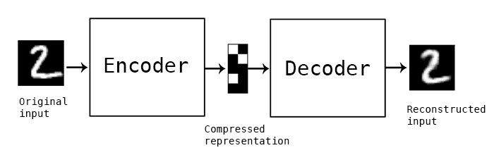
a simple AutoEncoder
1.1 AutoEncoder Components:
Autoencoders consists of 4 main parts:
-
Encoder: In which the model learns how to reduce the input dimensions and compress the input data into an encoded representation.
-
Bottleneck: which is the layer that contains the compressed representation of the input data. This is the lowest possible dimensions of the input data.
-
Decoder: In which the model learns how to reconstruct the data from the encoded representation to be as close to the original input as possible.
-
Reconstruction Loss: This is the method that measures measure how well the decoder is performing and how close the output is to the original input.
The training then involves using back propagation in order to minimize the network’s reconstruction loss. You must be wondering why would I train a neural network just to output an image or data that is exactly the same as the input! This article will cover the most common use cases for Autoencoder. Let’s get started:
\[Loss = \lVert X - \hat{X} \rVert_{2}^{2}\]1.2 Problem statement:
The network architecture for AutoEncoders can vary between a simple FeedForward network, LSTM network or Convolutional Neural Network depending on the use case. This article will use CNN networks to solve a simple problem. The problem is to remove an annoying text from the given picture. You might have seen that many photographic websites or some famous photographers use some texts as a sign or a signature on their images. That would prevent other people from stealing their valuable artistic photos, paintings, etc.
For example here is a sample photo taken by my psychologist friend Reza Parizi (reza__parizi):
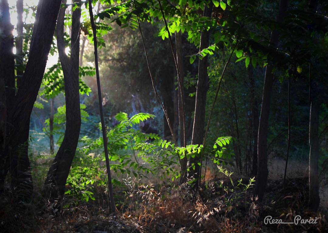
We can consider these kinds of texts which may be known by the name watermark as static noise in pictures. We can try to find a way or a set of filters to be applied to that image in order to remove that artifact. One of the main use cases of AutoEncoders is denoising, so let’s solve this problem using AutoEncoders.
2. Preparing the data:
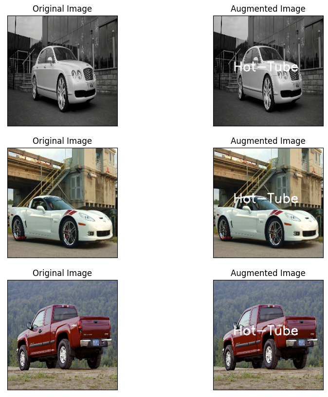
As you know for deep learning models the first thing we need is the data. For this problem, I used the popular Stanford cars dataset and I added the static text “Hot-Tube” to the images as the signature of the image. Let’s say that the data is stored in a directory named datasets/car and the training data is located inside another directory called train. First, we import all required modules:
import tensorflow as tf
import numpy as np
import keras
import keras.layers
import os
import matplotlib.pyplot as plt
import cv2
Then we have to load the dataset:
path_to_train_imgs = './datasets/cars/train'
train_imgs_list = os.listdir(path_to_train_imgs)
train_imgs_list = [f"{path_to_train_imgs}/{path}" for path in train_imgs_list]
These images are the original images which considered the ground truth. To generate the input data we have 2 ways:
- load all data into the memory and loop throw them adding the signature text.
- Write a DataGenerator which adds the signature to each image while creating the batch.
The first method is not always a good option, especially while working with images. because image data volumes are regularly high, loading this amount of data into the memory will cause the Out of memory problem and lead your programs to crash.
DataGenerators will load only that part of the data which is needed for the training on each period of time and it prevents the out-of-memory problem. After knowing the need for DataGenerators let’s write a DataGenerator for our program.
class DataGenerator(keras.utils.Sequence):
    def __init__(self, image_list, batch_size=16, shuffle=True):
        self.image_list = image_list
        self.batch_size = batch_size
        self.shuffle = shuffle
        self.on_epoch_end()

    def load_img(self, path: str) -> np:
        img = cv2.imread(path)
        img = cv2.cvtColor(img, cv2.COLOR_BGR2RGB)
        img = cv2.resize(img, (256,256))
        return img

    def on_epoch_end(self):
        self.indexes = np.arange(len(self.image_list))
        if self.shuffle == True:
            np.random.shuffle(self.indexes)

    def __len__(self):
        return len(self.image_list)//self.batch_size

    def add_text(self, img: np) -> np:
        return cv2.putText(img=img, text='Hot-Tube', org=(46, 128), fontFace=cv2.FONT_HERSHEY_SIMPLEX, fontScale=1, color=(255, 255, 255), thickness=2)

    def __getitem__(self, index):
        indexes = self.indexes[index*self.batch_size: (index+1)*self.batch_size]
        img_paths = [self.image_list[i] for i in indexes]

        Y = [self.load_img(img_path) for img_path in img_paths]
        X = [self.add_text(np.array(img)) for img in Y]

        return np.array(X)/255, np.array(Y)/255
Let’s see how it works:
def plt_img(img: np, title: str = None):
    plt.imshow(img)
    plt.xticks([])
    plt.yticks([])
    if title is not None:
        plt.title(title)

validation_imgs, train_imgs = train_imgs_list[:100], train_imgs_list[100:]
train_data_generator = DataGenerator(image_list=train_imgs)
validation_data_generator = DataGenerator(image_list=validation_imgs)

# Showing some sample images
X, Y = validation_data_generator[0]

plt.figure(figsize=(10,10))
cnt = 1;
for i in range(3):
    plt.subplot(3,2, cnt)
    plt_img(Y[i], "Original Image")
    cnt += 1
    plt.subplot(3, 2, cnt)
    plt_img(X[i], "Augmented Image")
    cnt += 1
plt.show()
3. Building the model
Let’s say that we have trained an autoencoder on the Cars dataset. Using a simple FeedForward neural network, we can achieve this by building a simple 9 layers network as below:
inputs = keras.layers.Input((256,256,3))
x = keras.layers.Conv2D(128, 3, padding='same', activation="relu")(inputs)
x = keras.layers.Conv2D(64, 3, padding='same', activation="relu")(inputs)
x = keras.layers.Conv2D(32, 3, padding='same', activation="relu")(inputs)
x = keras.layers.MaxPool2D()(x) # 128x128
x = keras.layers.Conv2D(8, 3, padding='same', activation="relu", name="bottle-neck")(x) # 128*128
x = keras.layers.UpSampling2D()(x) # 256x256
x = keras.layers.Conv2D(32, 3, padding='same', activation='relu')(x)
x = keras.layers.Conv2D(64, 3, padding='same', activation='relu')(x)
x = keras.layers.Conv2D(128, 3, padding='same', activation='relu')(x)
outputs = keras.layers.Conv2D(3, 1, padding='same', activation='relu')(x)

model = keras.Model(inputs, outputs)
model.compile(optimizer="adam", loss="mean_squared_error", metrics=['accuracy'])
model.summary()
Model: "model"
_________________________________________________________________
 Layer (type)                Output Shape              Param #
=================================================================
 input_1 (InputLayer)        [(None, 256, 256, 3)]     0

 conv2d_2 (Conv2D)           (None, 256, 256, 32)      896

 max_pooling2d (MaxPooling2D  (None, 128, 128, 32)     0
 )

 bottle-neck (Conv2D)        (None, 128, 128, 8)       2312

 up_sampling2d (UpSampling2D  (None, 256, 256, 8)      0
 )

 conv2d_3 (Conv2D)           (None, 256, 256, 32)      2336

 conv2d_4 (Conv2D)           (None, 256, 256, 64)      18496

 conv2d_5 (Conv2D)           (None, 256, 256, 128)     73856

 conv2d_6 (Conv2D)           (None, 256, 256, 3)       387

=================================================================
Total params: 98,283
Trainable params: 98,283
Non-trainable params: 0
_________________________________________________________________
I used mean squared error (MSE) loss to train my model. Because I wanted the model’s output to be the same as the original image. MSE should do the job for us perfectly but, we could use a different loss function that would compare the images from a regional point of view and would be better for high-resolution images and more general datasets. But, we are good with MSE on this task.
3.1 Tensorboard
To see how the training process is going on and monitor the training process, there is a useful option called Tensorboard developed by the TensorFlow team. Tensorboard is a background process that looks inside a directory (usually named “logs”) and visualizes the training process logs such as training and validation accuracy and loss for us. It also is capable to display images that can be generated during the training process such as model predictions at the end of each epoch. It would be so handy to store the model prediction during the training process. It could help us to find out when to terminate the training process in an experimental way.
To do so, we have to define a custom callback class to store model prediction on each epoch ended.
class TensorBoardImageCallBack(keras.callbacks.Callback):
    def __init__(self, log_dir, image, noisy_image):
        super().__init__()
        self.log_dir = log_dir
        self.image = image
        self.noisy_image = noisy_image

    def set_model(self, model):
        self.model = model
        self.writer = tf.summary.create_file_writer(self.log_dir, filename_suffix='images')

    def on_train_begin(self, _):
        self.write_image(self.noisy_image, 'Noisy Image', 0)
        self.write_image(self.image, 'Original Image', 0)

    def on_train_end(self, _):
        self.writer.close()

    def write_image(self, image, tag, epoch):
        image_to_write = np.copy(image)
        with self.writer.as_default():
            tf.summary.image(tag, image_to_write, step=epoch)

    def on_epoch_end(self, epoch, logs={}):
        denoised_image = self.model.predict_on_batch(self.noisy_image)
        self.write_image(denoised_image, 'Denoised Image', epoch)

tensorboard_callback = TensorBoardImageCallBack('./logs', Y[1:2], X[1:2])
tensorboard_callback_loss = tf.keras.callbacks.TensorBoard(log_dir="./logs")
3.2 Training the model
Now, it’s time to start training our model. I just hangup training the model after 25 epochs but, in code, I’ve defined the number of epochs to be 100. I hope continuing the training till 100 epochs will tend to a great convergence of the model.
history = model.fit(
            train_data_generator,
            epochs=100,
            validation_data=validation_data_generator,
            callbacks=[tensorboard_callback, tensorboard_callback_loss]
        )
...
502/502 [==============================] - 86s 171ms/step - loss: 6.6057e-04 - accuracy: 0.8184 - val_loss: 5.3678e-04 - val_accuracy: 0.8163
As you can see in the output, which is the results of training for about 25 epochs, the last reconstruction loss/error for the validation set is 5.3678e-04 which is great but it can be better if you run this code for about 100 epochs. Now, if I pass a new image from the test dataset, the reconstruction loss will be very low BUT if I tried to pass any other different image (outlier or anomaly), we will get a high reconstruction loss value because the network failed to reconstruct the image/input that is considered an anomaly, which is another use case of autoencoders to detect outlier data points.
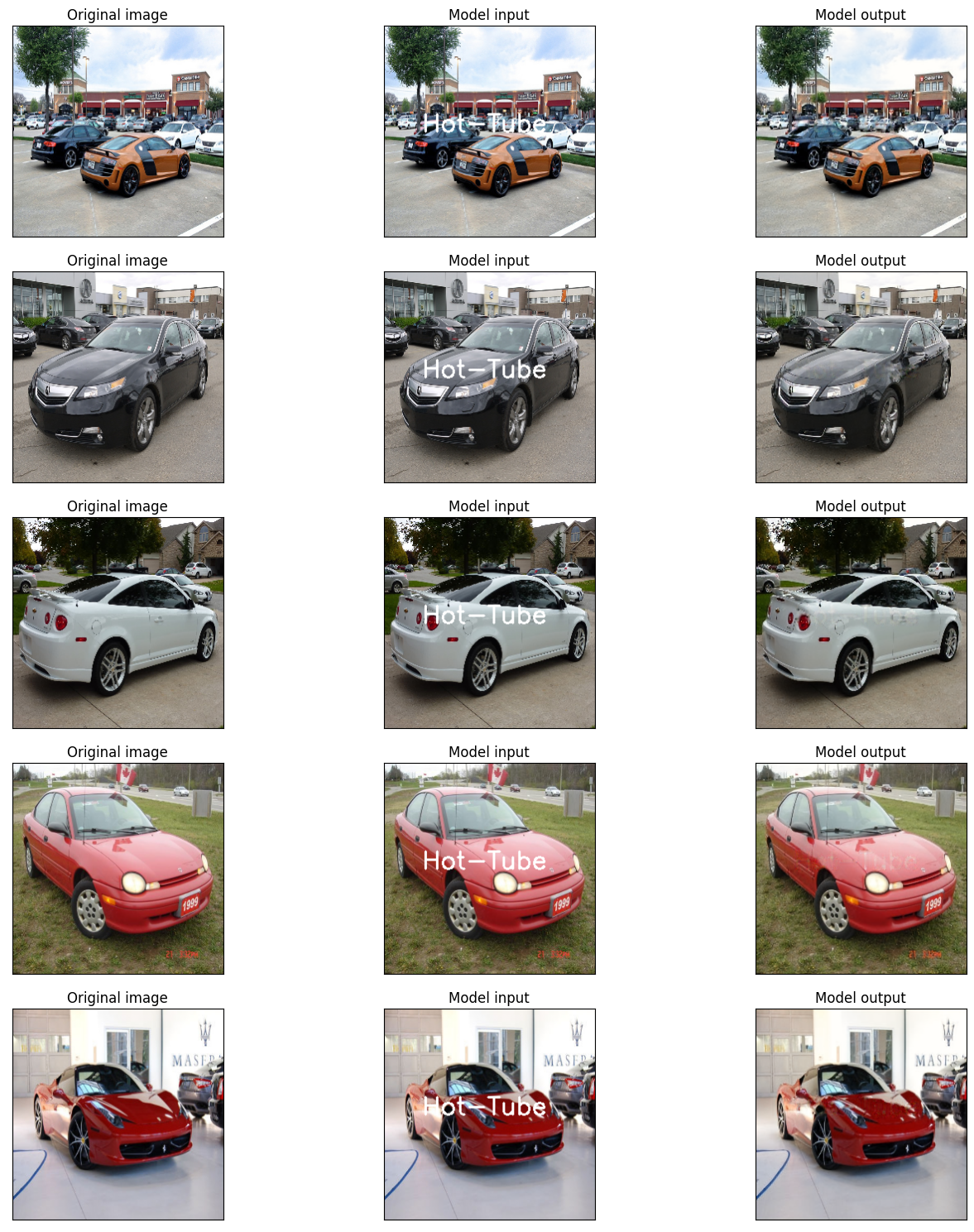
Notice in the code above, you can use only the encoder part to compress some data or images and you can also only use the decoder part to decompress the data by loading the decoder layers. As you can see, we reduced the input image dimensions from \(256 \times 256 \times 3\) to \(128 \times 128 \times 8\) which is accessible in the bottle-neck layer’s output. storing the features of this layer instead of the original images lowers the space needed to store the images by a factor of 1.5. If it was a video of size 900MB, using this technique would lead the size of the video to be 600MB which is more efficient for data storage.
\[\frac{256 \times 256 \times 3}{128 \times 128 \times 8} = 1.5\]
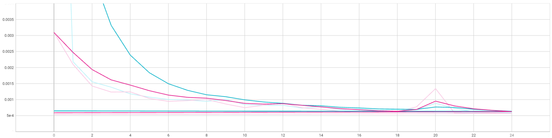
Model loss per epoch
Note: In the figure above, red is validation loss and the blue one is training loss per epoch.
Another use case of AutoEncoders is learning a data representation in lower dimensions which tends to data compression. Another cool use case is to enhance the quality of the picture which is called super-resolution which we can’t see on our model but I’ll do an experiment to implement super-resolution using AutoEncoders in another article.
Finally, we removed a static noise from the input data which is another use case of auto encoders we were follow. I hope you enjoyed reading my article. Stay tuned!
Comment Channel