
1. Intro
Knowing statistics for a computer engineer, a data scientist, or a machine-learning engineer is a unique need in their professional career. We learn about statistics in most universities more like learning differential equations or calculus instead. We know so many mathematical basics for statistics that we will never use in the future. That prevents us from seeing the use of statistics and what we can do with these concepts in the real world.
In this article, we are about to learn two crucial statistics concepts, The Poisson Distribution and The Poisson Process, through solving a common problem in the concept of online website hosting.
2. What Poisson Distribution or Poisson Process is about?
Before we get started, let’s first ask our selves a simple question, “Why do we need Poisson?”
The Poisson distribution helps us to o predict the probability of a given number of events occurring in a fixed interval of time, or just simply, to predict the number of events in the future.
For example,
- How many visitors do you get on your website in a day?
- How many clicks do your ads get for the next month?
- How many phone calls do you get during your shift?
- How many people will die from covid-19 next year?
Every week, on average, 17 people react to my blog posts via sending me emails. I’d like to predict the number of people who react to my blog posts next week because I have to consider some free time to answer them properly and planning is so critical for me.
What is the probability that exactly 20 people (or 10, 30, 40, etc.) will react to my posts next week?
To answer this question, if we knew some statistics, it would comes my our minds that we should be able to solve this problem using the Binomial distribution. Let’s first, look at the concept of Binomial distribution and solve the problem using it.
3. Binomial distribution
One way to solve this should be to start with the number of reads. Each person who reads the blog has some probability that they will really have a question or found some thing interesting to share with me.
A binomial random variable is the number of successes \(x\) in \(n\) repeated trials. And we assume the probability of success \(p\) is constant over each trial. The Binomial distribution formula is: \begin{equation} P[X=x] = \binom{n}{x}p^x(1-p)^{n-x} \end{equation}
However here, we are given only one piece of information, \(17 \frac{emails}{week}\), which is a rate. we don’t know any thing about the probability of receiving an email by an individual reader p, nor the number of blog visitors n. So, we use google analytics to retrieve this data from our blog history.
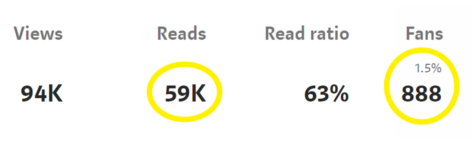
Stats from google
By looking to the stats we can say, in one year, A total of \(59k\) people read my blog. Out of \(59k\) people, \(888\) of them liked my post. Therefore, the number of people who read my blog per week (\(n\)) is \(\frac{59k}{52}=1134\). The number of people who liked my posts per week (\(x\)) is \(\frac{888}{52}=17\). So, the success probability p would be \(\frac{888}{59k} = 0.015\) or \(1.5\%\).
Now Using Binomial PMF, we should be able to calculate the probability of getting 20 emails for next week as below:
\[P[X=20] = \binom{1134}{20}(0.015)^{20}(1-0.015)^{n-x} = 0.06962\]We can use python or any other programming language to calculate the probability of getting emails with different values.
from scipy.stats import binom
# setting the values
# of n, p and x
n = 1134
p = 0.015
x_s = [10, 17, 20, 30, 40]

print(f"x\tBinomial P(x, n, p)")
print("----------------------------")
for x in x_s:
    print(f"{x}:\t{binom.pmf(x, n, p)}")
x	Binomial P(x, n, p)
----------------------------
10:	0.022507172903122208
17:	0.09701415708780352
20:	0.06962037106916726
30:	0.0012106250995813465
40:	6.815731666708672e-07
As you can see, by using binomial distribution the probability of getting, 10, 17, 20, 30 and 40 emails per week would be as follows:
| x | Binomial P(X=x) |
|---|---|
| 10 | 0.02250 |
| 17 | 0.09701 |
| 20 | 0.06962 |
| 30 | 0.00121 |
| 40 | < 0.000001 |
4. Shortcomings of the Binomial Distribution
The very first problem with a binomial random variable is, “it being assumed to be binary (0 or 1)”. In the previous example, we have \(17 \frac{emails}{week}\). This means \(\frac{17}{7}=2.4\) people will send me emails per day, and \(\frac{17}{7*24}\) = 0.1 people send me email per hour. If we model the success probability by hour (0.1 email/hr) using binomial random variable, this means most of the hours get zero emails but some hours will get exactly 1 email. However, it is also very possible that certain hours will get more that 1 email (2,3,5 emails, etc.) The problem with binomial is that it cannot contain more than 1 event in the unit of time (in this case, 1 hr is the unit time). The unit of time can only have 0 or 1 event.
How about dividing 1 hour into 60 minutes, and make unit time smaller, for example, a minute? If that so, then 1 hour can contain multiple events (Still, one minute will contain exactly one or zero events.). What if, during that one minute, we got multiple emails? (i.e someone shared your my blog post on Twitter and the traffic spiked at that minute.) Then what? We can divide a minute into seconds. then our time unit becomes a second and again a minute can contain multiple events. But this binary container problem will always exist for ever-smaller time units. The idea is, we can make the binomial random variable handle multiple events by dividing a unit time into smaller units. By using smaller divisions, we can make the original unit time contain more than one event. Mathematically, this means \(n\) goes to infinity. Since we assumed the rate is fixed, \(p\) must goes to zero. Because, when $n$ grows up to infinity,the number of intervals between the period becomes grows as $n$ and the probability of getting an email at each interval tends to be merely zero. In the other words, If $n$ goes to infinity, \(p\) should become zero, Other wise, \(np\), which is the number of events will blow up.
The second problem with the binomial random variable is, “when we want to use the binomial distribution, the number of trails, \(n\), and the probability of success, \(p\), should be known”. If you use Binomial, you cannot calculate the success probability only with the rate (i.e \(17\frac{emails}{week}\)). You need more information \(n\) and \(p\), in order to use the binomial PMF. The Poisson Distribution, on the other hand, doesn’t require you to know \(n\) or \(p\). We are assuming \(n\) is infinitely large (\(n\rightarrow\infty\)) and \(p\) is infinitesimal (\(p\rightarrow 0\)). The only parameter of the Poisson distribution is the rate \(\lambda\). (In real life only knowing the rate is much more common than knowing both \(n\) and \(p\))
5. Derive the poisson formula mathematically
Now, let’s deep dive into the binomial distribution formula with the assumption that we reached from the ideas of the previous section (Section 4). We find out that to solve the deal with the binary nature of the binomial random variable, we should increase the number of time units in our one week interval. Mathematically it means \(n\rightarrow\infty\):
\[P[X=x] = lim_{n\rightarrow\infty}\binom{n}{x}p^x(1-p)^{n-x}\]If, \(n\rightarrow\infty\) and \(p\rightarrow 0\) then we can assume that:
\[p = \frac{\lambda}{n}\]Then we have:
\[P[X=x] = lim_{n\rightarrow\infty}\binom{n}{x}(\frac{λ}{n})^x(1- (\frac{λ}{n}))^{n-x}\] \[\Rightarrow lim_{n\rightarrow\infty} \frac{n!}{(n-x)!x!}(\frac{λ}{n})^x(1- (\frac{λ}{n}))^{n-x}\] \[\Rightarrow lim_{n\rightarrow\infty} \frac{n!}{(n-x)!}\frac{1}{n^x}\frac{λ^x}{x!}(1-\frac{λ}{n})^n(1-\frac{λ}{n})^{-x}\] \[\Rightarrow lim_{n\rightarrow\infty} \frac{n!}{(n-x)!}\frac{1}{n^x}\frac{λ^x}{x!}e^{-λ}(1)\]Because:
\[lim_{n\rightarrow\infty}\frac{n!}{(n-x)!}\frac{1}{n^x} = 1\]We can say:
\begin{equation} P[X=x] = e^{-λ}\frac{λ^{x}}{x!} \end{equation}
Which is actually the Poisson random distribution formula.
6. Probability of events for a Poisson distribution
An event can occur 0, 1, 2, … times in an interval. The average number of events in an interval is designated λ. λ is the event rate. also called the rate parameter. The probability of observing k events in an interval is given by the equation:
\[P[k\ events\ in\ interval] = e^{-λ}\frac{λ^{k}}{k!}\]Where:
- \(\lambda\) is the average number of events per interval
- \(e\) is the number \(2.71828…\) (Euler’s number) the base of the natural logarithm
- \(k\) takes values \(0, 1, 2, …\)
- \(k! = k(k-1)(k-2)…(2)(1)\) is the factorial of \(k\)
We calculate the probability of observing 10, 17, 20, 30 and 40 emails in the interval using the poisson distribution formula as below:
from scipy.stats import poisson

#calculate probability

# setting the values
# of lambda and x
l = 17
x_s = [10, 17, 20, 30, 40]

print(f"x\tPoisson P(x, lambda)")
print("----------------------------")
for x in x_s:
    print(f"{x}:\t{poisson.pmf(k=x, mu=l)}")
x	Poisson P(x, lambda)
----------------------------
10:	0.022999584406166312
17:	0.09628462779844556
20:	0.06915882695522822
30:	0.001278796308921649
40:	8.381188233781985e-07
As it can be observed, using the calculated probabilities using Poisson formula is very close to the values calculated using Binomial distribution formula, so we can conclude that the Poisson distribution in this situation is a really good approximation for our problem. Because of the simpler formula and lower and easy to obtain parameter of the poisson distribution, it would be come very useful to use this distribution to solve the problems of this kind.
| x | Binomial P(X=x) | Poisson P(X=x;lambda=17) |
|---|---|---|
| 10 | 0.02250 | 0.2300 |
| 17 | 0.09701 | 0.09628 |
| 20 | 0.06962 | 0.07595 |
| 30 | 0.00121 | 0.00340 |
| 40 | < 0.000001 | < 0.000001 |
7. Some notes on Poisson random variable
Even though the Poisson distribution models are rare events, the rate \(\lambda\) can me any number. It doesn’t always have to be small. The Poisson Distribution is asymmetric, it is always skewed toward the right. Because it is inhibited by the zero occurrence barrier (there is no such thing as minus one email) on the left and it is unlimited on the other side. As \(\lambda\) becomes bigger, the graph looks more like a normal distribution.
from scipy.stats import poisson
import matplotlib.pyplot as plt

x_s = [i for i in range(0, 40, 5)]
plots = []
mus = [5, 10, 15, 17, 20]

for mu in mus:
  y_s = []
  for x in x_s:
    y_s += [poisson.pmf(k=x, mu=mu)]
  plots += [(x_s, y_s)]


plt.figure(figsize=(10,10))
for i in range(len(plots)):
  plt.plot(plots[i][0], plots[i][1], label=f"lambda = {mus[i]}")

plt.legend(loc='best')
plt.show()
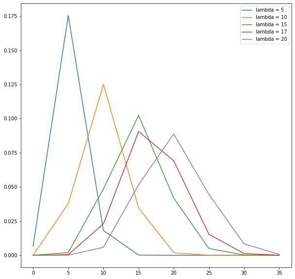
Poisson distribution with different lambda's for our problem.
The average rate of events per unit time in poisson distribution is constant. This means the number of people who visit my blog per hour might not follow a Poisson Distribution, because the hourly rate is not constant (higher rate during the daytime, lower rate during the night-time). Using monthly rate for consumer/biological data would be just an approximation as well, since the seasonality effect is non-trivial in that domain.
In poisson random variable, Events are independent. The arrival of my blog visitors might not always be independent. For example, sometimes a large number of visitors come in a group because someone popular mentioned my blog, or my blog got featured on Medium’s first page, etc. the number of earthquakes per year in a country also might not follow a Poisson Distribution in one large earthquake increases the probability of aftershocks.
Comment Channel