<?xml version="1.0" encoding="utf-8"?><feed xmlns="http://www.w3.org/2005/Atom" ><generator uri="https://jekyllrb.com/" version="4.2.2">Jekyll</generator><link href="https://alinaderiparizi.com/feed.xml" rel="self" type="application/atom+xml" /><link href="https://alinaderiparizi.com/" rel="alternate" type="text/html" /><updated>2026-09-28T21:30:43+00:00</updated><id>https://alinaderiparizi.com/feed.xml</id><title type="html">mralinp</title><subtitle>Ali Naderi: machine learning, medical imaging, embedded systems and the software around them.</subtitle><entry><title type="html">latex-academic-template: create-react-app for LaTeX</title><link href="https://alinaderiparizi.com/project/latex/docker/devtools/cli/2026/09/23/latex-academic-template.html" rel="alternate" type="text/html" title="latex-academic-template: create-react-app for LaTeX" /><published>2026-09-23T22:12:37+00:00</published><updated>2026-09-23T22:12:37+00:00</updated><id>https://alinaderiparizi.com/project/latex/docker/devtools/cli/2026/09/23/latex-academic-template</id><content type="html" xml:base="https://alinaderiparizi.com/project/latex/docker/devtools/cli/2026/09/23/latex-academic-template.html"><![CDATA[<p><a href="https://github.com/mralinp/latex-academic-template">latex-academic-template</a> started as the repo behind my own resume and turned into something more useful: a Dockerized LaTeX template gallery with a one-command scaffolding tool. No TeX Live install, no <code class="language-plaintext highlighter-rouge">tlmgr</code>, no losing an afternoon to a broken package manager. Getting from nothing to a compiling PDF is one command:</p>

<div class="language-bash highlighter-rouge"><div class="highlight"><pre class="highlight"><code>bash <span class="nt">-c</span> <span class="s2">"</span><span class="si">$(</span>curl <span class="nt">-fsSL</span> https://raw.githubusercontent.com/mralinp/latex-academic-template/main/create-latex-app.sh<span class="si">)</span><span class="s2">"</span>
</code></pre></div></div>

<p>This post is about why it exists, how the scaffolding wizard actually works, and two shell gotchas that only showed up once I stopped reading the script and started actually running it.</p>

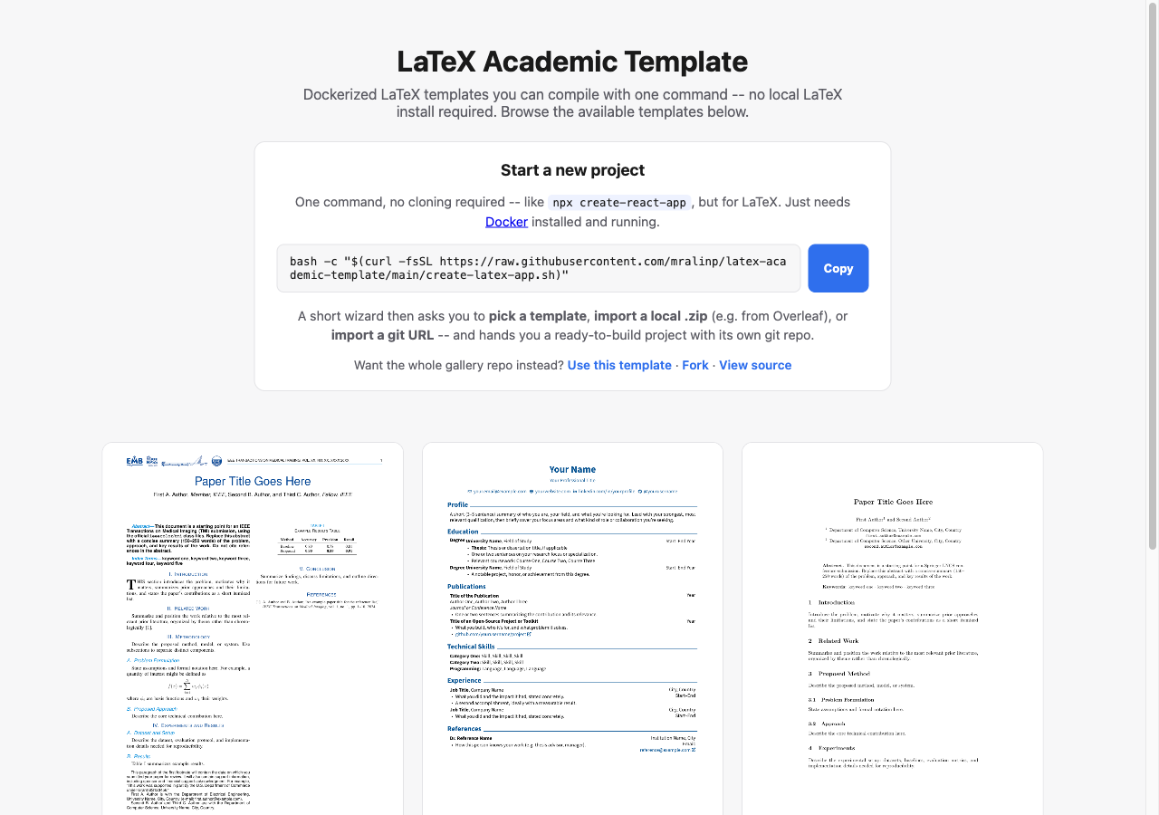
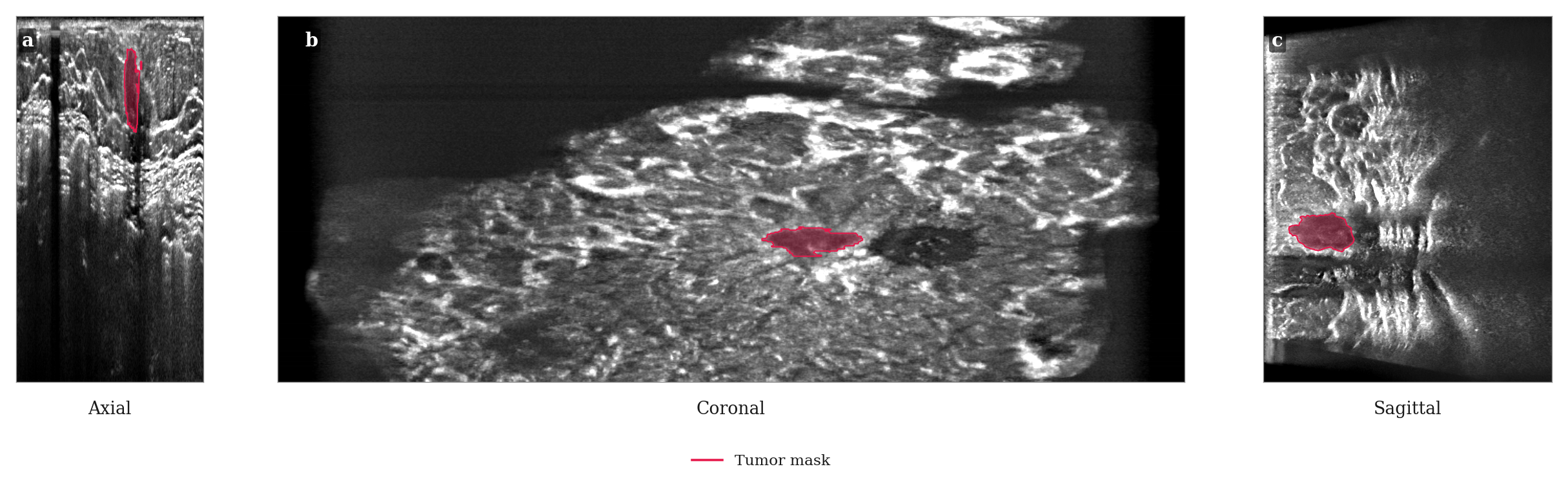
<p align="center">
    <img width="100%" src="/assets/images/posts/projects/latex-academic-template/gallery.png" />
</p>
<p align="center"><em>The live gallery: <a href="https://alinaderiparizi.com/latex-academic-template/">alinaderiparizi.com/latex-academic-template</a>.</em></p>

<h1 id="1-why">1. Why</h1>

<p>Every LaTeX document I write starts the same way: clone some old project, delete the content, keep the <code class="language-plaintext highlighter-rouge">\usepackage</code> block, and hope the machine I’m on still has the right TeX Live scheme installed. A full <code class="language-plaintext highlighter-rouge">scheme-full</code> install is several gigabytes and drifts out of sync between my laptop, my desktop, and CI the moment any of them updates independently. None of that has anything to do with actually writing the document.</p>

<p>The fix is the same one I already use for everything else: don’t install the toolchain, run it in a container. <code class="language-plaintext highlighter-rouge">docker-compose.yml</code> pulls the official <a href="https://hub.docker.com/r/texlive/texlive"><code class="language-plaintext highlighter-rouge">texlive/texlive</code></a> image, and a <code class="language-plaintext highlighter-rouge">Makefile</code> on top of it does the rest. The only two things a clone of this repo needs on the host machine are Docker and <code class="language-plaintext highlighter-rouge">make</code>, both of which are already sitting on any machine I do real work on.</p>

<h1 id="2-the-gallery">2. The gallery</h1>

<p>The repo is a <code class="language-plaintext highlighter-rouge">templates/</code> directory, one folder per document type, each with a <code class="language-plaintext highlighter-rouge">main.tex</code> and a small <code class="language-plaintext highlighter-rouge">config.mk</code> (engine, entry file, whether <code class="language-plaintext highlighter-rouge">-shell-escape</code> is needed). Three live there today:</p>

<ul>
  <li><strong>resume</strong> – a single-column CV with a contact-icon header built on <code class="language-plaintext highlighter-rouge">paracol</code> and <code class="language-plaintext highlighter-rouge">fontawesome5</code>.</li>
  <li><strong>ieee-transactions</strong> – the actual <a href="https://www.embs.org/tmi/">IEEE Transactions on Medical Imaging</a> author kit (<code class="language-plaintext highlighter-rouge">ieeecolor.cls</code> + <code class="language-plaintext highlighter-rouge">tmi.sty</code>), vendored directly since it isn’t on CTAN.</li>
  <li><strong>springer-lncs</strong> – a Springer Lecture Notes in Computer Science proceedings skeleton.</li>
</ul>

<p>Both the resume and the IEEE template used to be real content before I stripped them down. The IEEE one is a genericized version of the actual TMI draft for my <a href="/project/abus-classification/medical-imaging/ultrasound/mammography/breast-cancer/2026/09/16/abus-classification-1-imaging-modalities.html">spherical-harmonics ABUS work</a>; the class files, the footnote block, the <code class="language-plaintext highlighter-rouge">IEEEkeywords</code> environment, all of it came straight out of a real submission. Turning a working document into a template is a good forcing function: anything left in the placeholder version is there because it’s structurally useful, not because I forgot to delete it.</p>

<p>Adding a template is meant to be trivial:</p>

<div class="language-bash highlighter-rouge"><div class="highlight"><pre class="highlight"><code>make add-template <span class="nv">NAME</span><span class="o">=</span>ieee-conference
</code></pre></div></div>

<p>scaffolds <code class="language-plaintext highlighter-rouge">main.tex</code> and <code class="language-plaintext highlighter-rouge">config.mk</code>, and from that point it’s picked up automatically by <code class="language-plaintext highlighter-rouge">make list</code>, <code class="language-plaintext highlighter-rouge">make build-all</code>, and the gallery page. No registry file to edit.</p>

<h1 id="3-the-create-react-app-part">3. The <code class="language-plaintext highlighter-rouge">create-react-app</code> part</h1>

<p>The gallery on its own still meant cloning (or forking, or “Use this template”-ing) the whole multi-template repo just to write one document – correct, but not what most people actually want. What they want is closer to <code class="language-plaintext highlighter-rouge">npx create-react-app my-app</code>: one command, a couple of prompts, a working project. So <code class="language-plaintext highlighter-rouge">create-latex-app.sh</code> exists to do exactly that:</p>

<div class="language-bash highlighter-rouge"><div class="highlight"><pre class="highlight"><code>bash <span class="nt">-c</span> <span class="s2">"</span><span class="si">$(</span>curl <span class="nt">-fsSL</span> https://raw.githubusercontent.com/mralinp/latex-academic-template/main/create-latex-app.sh<span class="si">)</span><span class="s2">"</span>
</code></pre></div></div>

<p>It’s a plain bash script (bash 3.2-compatible, since that’s what macOS still ships), and it asks three things: a project name, then one of</p>

<ul>
  <li><strong>a gallery template</strong> (resume, IEEE, Springer, …),</li>
  <li><strong>a local <code class="language-plaintext highlighter-rouge">.zip</code></strong>, e.g. exported straight out of Overleaf, or</li>
  <li><strong>a git URL</strong>, e.g. an Overleaf project’s git remote,</li>
</ul>

<p>and hands back a standalone folder with its own minimal <code class="language-plaintext highlighter-rouge">Makefile</code>, <code class="language-plaintext highlighter-rouge">docker-compose.yml</code>, and a fresh git repo with an initial commit, offering to run the first build immediately. For the <code class="language-plaintext highlighter-rouge">.zip</code>/git-import paths it also auto-detects the entry <code class="language-plaintext highlighter-rouge">.tex</code> file (first <code class="language-plaintext highlighter-rouge">main.tex</code> it finds, otherwise the first file with both <code class="language-plaintext highlighter-rouge">\documentclass</code> and <code class="language-plaintext highlighter-rouge">\begin{document}</code>) and, if the imported project already has its own <code class="language-plaintext highlighter-rouge">Makefile</code> or <code class="language-plaintext highlighter-rouge">README</code>, backs the originals up instead of silently overwriting them.</p>

<p>It also runs locally as <code class="language-plaintext highlighter-rouge">make create</code> for anyone already sitting inside a clone.</p>

<h1 id="4-two-bugs-that-only-existed-at-runtime">4. Two bugs that only existed at runtime</h1>

<p><strong>A source that hadn’t fully synced produced a fake success.</strong> Early on I tested the script against the just-pushed repo before the push had actually landed, so the temp clone it made was missing <code class="language-plaintext highlighter-rouge">scaffold/Makefile</code>. The <code class="language-plaintext highlighter-rouge">cp</code> failed, the <code class="language-plaintext highlighter-rouge">sed</code> failed, and the script kept going anyway and printed “Created my-project/” like nothing had happened – because nothing in it actually checked that the pieces it depended on were there. The fix was a <code class="language-plaintext highlighter-rouge">verify_source()</code> step, run right after the clone and before anything is written to disk, that fails loudly if the expected files aren’t present. Obvious in hindsight; invisible until I ran it against a source that was actually broken instead of one I’d manually pre-verified.</p>

<p><strong><code class="language-plaintext highlighter-rouge">bash -c "$(curl ...)" arg1 arg2</code> doesn’t do what it looks like it does.</strong> The README’s documented one-liner works fine with no arguments. The moment I tried to pass flags through it the same way –</p>

<div class="language-bash highlighter-rouge"><div class="highlight"><pre class="highlight"><code>bash <span class="nt">-c</span> <span class="s2">"</span><span class="si">$(</span>curl <span class="nt">-fsSL</span> .../create-latex-app.sh<span class="si">)</span><span class="s2">"</span> my-cv <span class="nt">--template</span> resume
</code></pre></div></div>

<p>– it hung. Turns out <code class="language-plaintext highlighter-rouge">bash -c command_string arg0 arg1 ...</code> assigns the <em>first</em> trailing argument to <code class="language-plaintext highlighter-rouge">$0</code>, not <code class="language-plaintext highlighter-rouge">$1</code>. <code class="language-plaintext highlighter-rouge">my-cv</code> silently became the script’s <code class="language-plaintext highlighter-rouge">$0</code> and vanished; the actual arguments the script saw were just <code class="language-plaintext highlighter-rouge">--template resume</code>, so the project name was never set, and it sat blocked on a <code class="language-plaintext highlighter-rouge">read</code> prompt that had no terminal left to answer it, since stdin had already been consumed by the command substitution. The fix isn’t in the script – it’s a documentation problem, the same one <code class="language-plaintext highlighter-rouge">rustup</code> and a few other curl-installers solve the same way: pass a throwaway placeholder for <code class="language-plaintext highlighter-rouge">$0</code>.</p>

<div class="language-bash highlighter-rouge"><div class="highlight"><pre class="highlight"><code>bash <span class="nt">-c</span> <span class="s2">"</span><span class="si">$(</span>curl <span class="nt">-fsSL</span> .../create-latex-app.sh<span class="si">)</span><span class="s2">"</span> _ my-cv <span class="nt">--template</span> resume
</code></pre></div></div>

<p>Neither of these would have surfaced from reading the script. They only showed up once I ran the exact commands I was telling people to run, against the actual published repo instead of a local copy.</p>

<h1 id="5-whats-next">5. What’s next</h1>

<p>The Makefile is deliberately more than <code class="language-plaintext highlighter-rouge">build</code>: <code class="language-plaintext highlighter-rouge">watch</code> (<code class="language-plaintext highlighter-rouge">latexmk -pvc</code>), <code class="language-plaintext highlighter-rouge">lint</code> (<code class="language-plaintext highlighter-rouge">chktex</code>), <code class="language-plaintext highlighter-rouge">wordcount</code> (<code class="language-plaintext highlighter-rouge">texcount</code>), <code class="language-plaintext highlighter-rouge">clean</code>/<code class="language-plaintext highlighter-rouge">clean-all</code>, <code class="language-plaintext highlighter-rouge">shell</code> to drop into the container directly. CI builds every template on every push, and a GitHub Pages workflow renders a thumbnail of each one’s first page and republishes the gallery you see above – all inside the same container, so the preview is never out of sync with what <code class="language-plaintext highlighter-rouge">make build</code> actually produces.</p>

<p>The template list is intentionally short right now. IEEE Transactions and Springer LNCS were the two I actually needed; more will show up the same way those did, as real documents that get stripped down once they’re not needed as drafts anymore.</p>

<p>If you want a LaTeX document without installing LaTeX, <code class="language-plaintext highlighter-rouge">bash -c "$(curl -fsSL https://raw.githubusercontent.com/mralinp/latex-academic-template/main/create-latex-app.sh)"</code> and see what it gives you. Issues and template contributions are welcome on <a href="https://github.com/mralinp/latex-academic-template">GitHub</a>.</p>]]></content><author><name>Ali Naderi</name></author><category term="project" /><category term="latex" /><category term="docker" /><category term="devtools" /><category term="cli" /><summary type="html"><![CDATA[latex-academic-template started as the repo behind my own resume and turned into something more useful: a Dockerized LaTeX template gallery with a one-command scaffolding tool. No TeX Live install, no tlmgr, no losing an afternoon to a broken package manager. Getting from nothing to a compiling PDF is one command:]]></summary></entry><entry><title type="html">tdsc-abus2023-pytorch: A PyTorch Dataset for 3D Breast Ultrasound</title><link href="https://alinaderiparizi.com/project/abus-classification/medical-imaging/pytorch/python/2026/09/23/tdsc-abus2023-pytorch.html" rel="alternate" type="text/html" title="tdsc-abus2023-pytorch: A PyTorch Dataset for 3D Breast Ultrasound" /><published>2026-09-23T06:30:00+00:00</published><updated>2026-09-23T06:30:00+00:00</updated><id>https://alinaderiparizi.com/project/abus-classification/medical-imaging/pytorch/python/2026/09/23/tdsc-abus2023-pytorch</id><content type="html" xml:base="https://alinaderiparizi.com/project/abus-classification/medical-imaging/pytorch/python/2026/09/23/tdsc-abus2023-pytorch.html"><![CDATA[<p><a href="https://github.com/mralinp/tdsc-abus2023-pytorch">tdsc-abus2023-pytorch</a> is the data layer under my <a href="/project/abus-classification/medical-imaging/ultrasound/mammography/breast-cancer/2026/09/16/abus-classification-1-imaging-modalities.html">ABUS classification</a> project. It’s a PyTorch <code class="language-plaintext highlighter-rouge">Dataset</code> for the TDSC-ABUS 2023 challenge [1]: 200 automated 3D breast ultrasound volumes, each with a tumor mask, a bounding box, and a malignant/benign label. It’s on PyPI, so getting from nothing to a training loop is one line:</p>

<div class="language-bash highlighter-rouge"><div class="highlight"><pre class="highlight"><code>pip <span class="nb">install </span>tdsc-abus2023-pytorch
</code></pre></div></div>

<p>This post is about why it exists, what it does, and what I had to fix to make it trustworthy, which turned out to be most of the work.</p>

<p align="center">
    <img width="60%" src="/assets/images/posts/projects/tdsc-abus2023-pytorch/sample_case.png" />
</p>
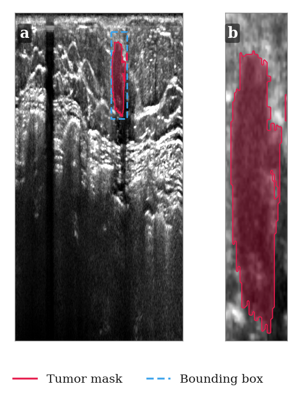
<p align="center"><em>Case 8 (malignant). (a) Axial slice of the full volume from <code>TDSC</code>, with the tumor mask and bounding box. (b) The same tumor from <code>TDSCTumors</code>, cropped to its bounding box.</em></p>

<h1 id="1-why-a-package-at-all">1. Why a package at all</h1>

<p>The challenge data ships as <code class="language-plaintext highlighter-rouge">.nrrd</code> volumes plus two CSVs per split: <code class="language-plaintext highlighter-rouge">labels.csv</code> (case id, label, file paths) and <code class="language-plaintext highlighter-rouge">bbx_labels.csv</code> (bounding-box centre and size). Every project that uses it ends up writing the same glue: download the zips from Google Drive, unzip them, parse the CSVs, read the NRRD files, turn <code class="language-plaintext highlighter-rouge">'M'</code>/<code class="language-plaintext highlighter-rouge">'B'</code> into integers, and convert centre-plus-size boxes into corner coordinates. I’d written that glue three times across experiments before I gave up and put it in a package.</p>

<p>The dataset itself is summarized below. Volumes are big, around 843×546×270 to 865×682×354 voxels, and the voxels aren’t cubes: about 0.2 × 0.073 mm in-plane and ~0.476 mm between slices.</p>

<table>
  <thead>
    <tr>
      <th>Split</th>
      <th style="text-align: right">Cases</th>
      <th style="text-align: right">Malignant</th>
      <th style="text-align: right">Benign</th>
    </tr>
  </thead>
  <tbody>
    <tr>
      <td>Train</td>
      <td style="text-align: right">100</td>
      <td style="text-align: right">58</td>
      <td style="text-align: right">42</td>
    </tr>
    <tr>
      <td>Validation</td>
      <td style="text-align: right">30</td>
      <td style="text-align: right">17</td>
      <td style="text-align: right">13</td>
    </tr>
    <tr>
      <td>Test</td>
      <td style="text-align: right">70</td>
      <td style="text-align: right">40</td>
      <td style="text-align: right">30</td>
    </tr>
  </tbody>
</table>

<h1 id="2-what-you-get">2. What you get</h1>

<p>Two dataset classes. <code class="language-plaintext highlighter-rouge">TDSC</code> gives you the full volume:</p>

<div class="language-python highlighter-rouge"><div class="highlight"><pre class="highlight"><code><span class="kn">from</span> <span class="nn">tdsc_abus2023_pytorch</span> <span class="kn">import</span> <span class="n">TDSC</span><span class="p">,</span> <span class="n">DataSplits</span>

<span class="n">dataset</span> <span class="o">=</span> <span class="n">TDSC</span><span class="p">(</span><span class="n">path</span><span class="o">=</span><span class="s">"./data"</span><span class="p">,</span> <span class="n">split</span><span class="o">=</span><span class="n">DataSplits</span><span class="p">.</span><span class="n">TRAIN</span><span class="p">,</span> <span class="n">download</span><span class="o">=</span><span class="bp">True</span><span class="p">)</span>
<span class="n">volume</span><span class="p">,</span> <span class="n">mask</span><span class="p">,</span> <span class="n">label</span><span class="p">,</span> <span class="n">bbox</span> <span class="o">=</span> <span class="n">dataset</span><span class="p">[</span><span class="mi">0</span><span class="p">]</span>
</code></pre></div></div>

<p><code class="language-plaintext highlighter-rouge">label</code> is <code class="language-plaintext highlighter-rouge">0</code> for malignant and <code class="language-plaintext highlighter-rouge">1</code> for benign, and <code class="language-plaintext highlighter-rouge">bbox</code> is <code class="language-plaintext highlighter-rouge">((x0, y0, z0), (x1, y1, z1))</code> in the volume’s native coordinates. With <code class="language-plaintext highlighter-rouge">download=True</code>, the split is fetched and extracted on first use. After that it stays on disk and nothing touches the network.</p>

<p><code class="language-plaintext highlighter-rouge">TDSCTumors</code> returns the same thing already cropped to the tumor’s bounding box. For classification that’s usually what you want: the tumor is a small fraction of the volume, and there’s no reason to carry the rest of the breast through the pipeline.</p>

<div class="language-python highlighter-rouge"><div class="highlight"><pre class="highlight"><code><span class="kn">from</span> <span class="nn">tdsc_abus2023_pytorch</span> <span class="kn">import</span> <span class="n">TDSCTumors</span>

<span class="n">dataset</span> <span class="o">=</span> <span class="n">TDSCTumors</span><span class="p">(</span><span class="n">path</span><span class="o">=</span><span class="s">"./data"</span><span class="p">,</span> <span class="n">split</span><span class="o">=</span><span class="s">"Train"</span><span class="p">,</span> <span class="n">download</span><span class="o">=</span><span class="bp">True</span><span class="p">)</span>
<span class="n">volume</span><span class="p">,</span> <span class="n">mask</span><span class="p">,</span> <span class="n">label</span> <span class="o">=</span> <span class="n">dataset</span><span class="p">[</span><span class="mi">0</span><span class="p">]</span>
</code></pre></div></div>

<p>Transforms are plain callables <code class="language-plaintext highlighter-rouge">(volume, mask) -&gt; (volume, mask)</code>, applied in order. The only one the package ships is <code class="language-plaintext highlighter-rouge">ViewTransformer</code>, which transposes the volume into the axial, coronal or sagittal plane. As <a href="/project/abus-classification/medical-imaging/ultrasound/mammography/breast-cancer/2026/09/16/abus-classification-1-imaging-modalities.html">Part 1</a> explains, the coronal plane is the one handheld ultrasound never captures and the one where spiculation shows up best, so switching views is a one-line change on purpose:</p>

<div class="language-python highlighter-rouge"><div class="highlight"><pre class="highlight"><code><span class="kn">from</span> <span class="nn">tdsc_abus2023_pytorch</span> <span class="kn">import</span> <span class="n">ViewTransformer</span><span class="p">,</span> <span class="n">ViewTransposeConfig</span>

<span class="n">dataset</span> <span class="o">=</span> <span class="n">TDSC</span><span class="p">(</span>
    <span class="n">path</span><span class="o">=</span><span class="s">"./data"</span><span class="p">,</span>
    <span class="n">split</span><span class="o">=</span><span class="n">DataSplits</span><span class="p">.</span><span class="n">TRAIN</span><span class="p">,</span>
    <span class="n">transforms</span><span class="o">=</span><span class="p">[</span><span class="n">ViewTransformer</span><span class="p">(</span><span class="n">view</span><span class="o">=</span><span class="n">ViewTransposeConfig</span><span class="p">.</span><span class="n">CORONAL</span><span class="p">)],</span>
<span class="p">)</span>
</code></pre></div></div>

<p align="center">
    <img width="100%" src="/assets/images/posts/projects/tdsc-abus2023-pytorch/views.png" />
</p>
<p align="center"><em>The same tumor through each view <code>ViewTransformer</code> produces: (a) axial, (b) coronal, (c) sagittal.</em></p>

<p>The dependency list is deliberately short: <code class="language-plaintext highlighter-rouge">torch</code>, <code class="language-plaintext highlighter-rouge">numpy</code>, <code class="language-plaintext highlighter-rouge">pandas</code>, <code class="language-plaintext highlighter-rouge">pynrrd</code> and <code class="language-plaintext highlighter-rouge">gdown</code>.</p>

<h1 id="3-the-bugs-that-were-hiding-in-it">3. The bugs that were hiding in it</h1>

<p>The first version, from March 2025, worked on my machine and for my experiments. When I went back through it properly this month, I found that “worked” was doing a lot of the lifting.</p>

<p><strong><code class="language-plaintext highlighter-rouge">TDSCTumors</code> transformed twice and cropped in the wrong place.</strong> It called the parent’s <code class="language-plaintext highlighter-rouge">__getitem__</code>, which already applied the transforms, then cropped using the bounding box, then applied the transforms <em>again</em>. The bounding box is defined in the original coordinate space, so with a <code class="language-plaintext highlighter-rouge">ViewTransformer</code> in the list the crop was taken from a transposed volume using untransposed coordinates. You got a region of the right size from the wrong part of the breast, and nothing crashed. That’s the worst kind of bug in a data pipeline: the model trains, the loss goes down, and the data is wrong. The fix was a <code class="language-plaintext highlighter-rouge">_get_raw_item()</code> that loads without transforms. <code class="language-plaintext highlighter-rouge">TDSCTumors</code> now crops first and transforms once, and there’s a regression test that fails if either ordering comes back.</p>

<p><strong>It claimed Python 3.7 support and couldn’t import on it.</strong> The type hints used <code class="language-plaintext highlighter-rouge">X | Y</code> unions, which raise at import time before Python 3.10. A <code class="language-plaintext highlighter-rouge">from __future__ import annotations</code> fixed that, and the minimum is now an honest 3.9.</p>

<p><strong>The download metadata was never actually packaged.</strong> The Google Drive file list was bundled with the package, but the code ignored it and fetched a copy from GitHub over HTTP. That relied on <code class="language-plaintext highlighter-rouge">requests</code>, which was never declared and was only installed because <code class="language-plaintext highlighter-rouge">gdown</code> pulls it in. Separately, <code class="language-plaintext highlighter-rouge">MANIFEST.in</code> pointed at a path with hyphens instead of underscores, so the bundled file wasn’t in the wheel either. Now it’s read with <code class="language-plaintext highlighter-rouge">importlib.resources</code> and ships with the package.</p>

<p><strong>The tests downloaded several gigabytes every run.</strong> Every test used <code class="language-plaintext highlighter-rouge">download=True</code> with nothing mocked, and <code class="language-plaintext highlighter-rouge">pytest.ini</code> measured coverage of a module named <code class="language-plaintext highlighter-rouge">tdsc</code> that doesn’t exist, so the coverage report was measuring nothing. The suite now builds a tiny synthetic NRRD/CSV dataset in a fixture and runs offline in seconds.</p>

<p>None of these were hard to fix. They were just invisible until I stopped using the code and started reading it.</p>

<h1 id="4-making-loading-fast">4. Making loading fast</h1>

<p>Here’s the problem that bothered me most in practice. The volumes are gzip-compressed NRRD, so every <code class="language-plaintext highlighter-rouge">dataset[i]</code> decompresses roughly 200 MB, even in <code class="language-plaintext highlighter-rouge">TDSCTumors</code>, where you then throw away almost all of it to keep a crop a few centimetres across. Over many epochs with several DataLoader workers, that’s a lot of CPU spent unzipping the same bytes again and again.</p>

<p>The fix is an opt-in <code class="language-plaintext highlighter-rouge">cache=True</code>:</p>

<div class="language-python highlighter-rouge"><div class="highlight"><pre class="highlight"><code><span class="n">dataset</span> <span class="o">=</span> <span class="n">TDSCTumors</span><span class="p">(</span><span class="n">path</span><span class="o">=</span><span class="s">"./data"</span><span class="p">,</span> <span class="n">split</span><span class="o">=</span><span class="n">DataSplits</span><span class="p">.</span><span class="n">TRAIN</span><span class="p">,</span> <span class="n">cache</span><span class="o">=</span><span class="bp">True</span><span class="p">)</span>
<span class="n">loader</span> <span class="o">=</span> <span class="n">torch</span><span class="p">.</span><span class="n">utils</span><span class="p">.</span><span class="n">data</span><span class="p">.</span><span class="n">DataLoader</span><span class="p">(</span><span class="n">dataset</span><span class="p">,</span> <span class="n">batch_size</span><span class="o">=</span><span class="mi">1</span><span class="p">,</span> <span class="n">num_workers</span><span class="o">=</span><span class="mi">4</span><span class="p">)</span>
</code></pre></div></div>

<p>On first access, each NRRD is decompressed once and saved as an uncompressed <code class="language-plaintext highlighter-rouge">.npy</code> next to it. Every later read opens that file with <code class="language-plaintext highlighter-rouge">np.load(..., mmap_mode="r")</code>. That has three effects:</p>

<ul>
  <li><code class="language-plaintext highlighter-rouge">TDSC</code> skips decompression entirely.</li>
  <li><code class="language-plaintext highlighter-rouge">TDSCTumors</code> slices the memmap, so the OS only reads the pages under the tumor’s bounding box instead of the whole volume.</li>
  <li>DataLoader workers share the OS page cache, so four workers don’t mean four private copies of the same volume in RAM.</li>
</ul>

<p>It costs about 1.5× the NRRD’s disk space, which is why it’s off by default. The one subtle part is concurrency: several workers can hit the same uncached file at the same moment. Each worker writes to its own <code class="language-plaintext highlighter-rouge">&lt;name&gt;.npy.&lt;pid&gt;.tmp</code> and then <code class="language-plaintext highlighter-rouge">os.replace</code>s it into place. The rename is atomic, so no worker ever memory-maps a half-written file.</p>

<div class="language-python highlighter-rouge"><div class="highlight"><pre class="highlight"><code><span class="k">if</span> <span class="ow">not</span> <span class="n">os</span><span class="p">.</span><span class="n">path</span><span class="p">.</span><span class="n">exists</span><span class="p">(</span><span class="n">npy_path</span><span class="p">):</span>
    <span class="n">volume</span><span class="p">,</span> <span class="n">_</span> <span class="o">=</span> <span class="n">nrrd</span><span class="p">.</span><span class="n">read</span><span class="p">(</span><span class="n">full_path</span><span class="p">)</span>
    <span class="n">tmp_path</span> <span class="o">=</span> <span class="sa">f</span><span class="s">"</span><span class="si">{</span><span class="n">npy_path</span><span class="si">}</span><span class="s">.</span><span class="si">{</span><span class="n">os</span><span class="p">.</span><span class="n">getpid</span><span class="p">()</span><span class="si">}</span><span class="s">.tmp"</span>
    <span class="k">with</span> <span class="nb">open</span><span class="p">(</span><span class="n">tmp_path</span><span class="p">,</span> <span class="s">"wb"</span><span class="p">)</span> <span class="k">as</span> <span class="n">f</span><span class="p">:</span>
        <span class="n">np</span><span class="p">.</span><span class="n">save</span><span class="p">(</span><span class="n">f</span><span class="p">,</span> <span class="n">volume</span><span class="p">)</span>
    <span class="n">os</span><span class="p">.</span><span class="n">replace</span><span class="p">(</span><span class="n">tmp_path</span><span class="p">,</span> <span class="n">npy_path</span><span class="p">)</span>
<span class="k">return</span> <span class="n">np</span><span class="p">.</span><span class="n">load</span><span class="p">(</span><span class="n">npy_path</span><span class="p">,</span> <span class="n">mmap_mode</span><span class="o">=</span><span class="s">"r"</span><span class="p">)</span>
</code></pre></div></div>

<p><code class="language-plaintext highlighter-rouge">TDSCTumors</code> also copies its crop out of the memmap with <code class="language-plaintext highlighter-rouge">np.array(...)</code> right away, so the full volume’s mapping can be released as soon as the crop is taken, instead of living as long as the sample does.</p>

<h1 id="5-shipping-it">5. Shipping it</h1>

<p>The last piece was release plumbing. Publishing used to fail whenever a push to <code class="language-plaintext highlighter-rouge">main</code> reused a version number that was already on PyPI. CI now looks up the latest published version and bumps the patch number automatically, unless I’ve already bumped it by hand past that. The version lives in exactly one place, <code class="language-plaintext highlighter-rouge">__version__</code>, and <code class="language-plaintext highlighter-rouge">setup.py</code> reads it from there. Pushes to <code class="language-plaintext highlighter-rouge">main</code> go straight to stable PyPI, and other branches build but never publish.</p>

<h1 id="6-whats-next">6. What’s next</h1>

<p>The package is intentionally boring: load the data correctly, load it fast, and get out of the way. The interesting work happens on top of it in the <a href="https://github.com/mralinp/abus-classification">abus-classification</a> series. The next posts there cover the classical radiology features we reproduce as a baseline, and then the deep-learning models, all of them reading their data through <code class="language-plaintext highlighter-rouge">TDSCTumors</code>.</p>

<p>If you’re working on TDSC-ABUS, <code class="language-plaintext highlighter-rouge">pip install tdsc-abus2023-pytorch</code> and please cite the challenge paper [1]. Issues and PRs are welcome on <a href="https://github.com/mralinp/tdsc-abus2023-pytorch">GitHub</a>.</p>

<h1 id="references">References</h1>

<ol>
  <li>G. Luo et al. Tumor Detection, Segmentation and Classification Challenge on Automated 3D Breast Ultrasound: The TDSC-ABUS Challenge. arXiv:2501.15588, 2025. <a href="https://arxiv.org/abs/2501.15588">arxiv.org/abs/2501.15588</a></li>
</ol>]]></content><author><name>Ali Naderi</name></author><category term="project" /><category term="abus-classification" /><category term="medical-imaging" /><category term="pytorch" /><category term="python" /><summary type="html"><![CDATA[tdsc-abus2023-pytorch is the data layer under my ABUS classification project. It’s a PyTorch Dataset for the TDSC-ABUS 2023 challenge [1]: 200 automated 3D breast ultrasound volumes, each with a tumor mask, a bounding box, and a malignant/benign label. It’s on PyPI, so getting from nothing to a training loop is one line:]]></summary></entry><entry><title type="html">ABUS Classification, Part 1: Mammography, Ultrasound, and Why 3D</title><link href="https://alinaderiparizi.com/project/abus-classification/medical-imaging/ultrasound/mammography/breast-cancer/2026/09/16/abus-classification-1-imaging-modalities.html" rel="alternate" type="text/html" title="ABUS Classification, Part 1: Mammography, Ultrasound, and Why 3D" /><published>2026-09-16T06:30:00+00:00</published><updated>2026-09-16T06:30:00+00:00</updated><id>https://alinaderiparizi.com/project/abus-classification/medical-imaging/ultrasound/mammography/breast-cancer/2026/09/16/abus-classification-1-imaging-modalities</id><content type="html" xml:base="https://alinaderiparizi.com/project/abus-classification/medical-imaging/ultrasound/mammography/breast-cancer/2026/09/16/abus-classification-1-imaging-modalities.html"><![CDATA[<p>This is the first post of a series following <a href="https://alinaderiparizi.com/abus-classification/">abus-classification</a>, a project classifying malignant and benign breast lesions in 3D automated breast ultrasound (ABUS). I’ll add one post per phase of the project — this one is background, with no results yet: what a breast tumor is, how it gets imaged, and why this project uses 3D ultrasound specifically. The next post covers the classical radiology features we reproduce as a baseline; the one after that covers the deep-learning approaches.</p>

<h1 id="1-what-were-actually-looking-for">1. What we’re actually looking for</h1>

<p>A breast tumor is a mass of tissue that grows where it shouldn’t. Most breast masses are benign — fibroadenomas, cysts, areas of fibrocystic change — and are not life-threatening. The ones that matter are malignant: cancer cells that, left alone, can invade surrounding tissue and spread elsewhere in the body. The entire point of breast imaging is to find a mass and estimate, without cutting the patient open, whether it’s one or the other.</p>

<p>Imaging alone cannot give a definitive answer. A mammogram or an ultrasound scan produces an image that a radiologist scores on the BI-RADS scale, from “definitely benign” to “highly suggestive of malignancy” — a risk estimate, not a diagnosis. The only way to know for certain is a biopsy: a small sample of tissue examined under a microscope by a pathologist. What imaging is for is deciding <em>who needs a biopsy in the first place</em>, and increasingly, helping the radiologist read the image faster and more consistently. That second role — computer-aided reading — is what this project is ultimately building toward.</p>

<h1 id="2-two-very-different-ways-to-make-an-image">2. Two very different ways to make an image</h1>

<p>Mammography and ultrasound solve the same problem — see inside the breast without surgery — using completely different physics, and that’s why they see different things.</p>

<p><strong>Mammography</strong> sends X-rays through the compressed breast and records how much of each ray gets absorbed on the way through. Denser tissue (glandular and fibrous tissue, and tumors, which tend to be denser than surrounding fat) absorbs more X-rays and shows up brighter; fat absorbs little and shows up dark. It’s a projection, like a shadow: the whole breast thickness is compressed into one flat 2D image (two, usually — craniocaudal and mediolateral-oblique views, to get some sense of depth by triangulation). Mammography is very good at one thing in particular: <strong>microcalcifications</strong>, tiny calcium deposits as small as a fraction of a millimetre, which show up as bright specks and are an early sign of some cancers, well before a mass is large enough to feel.</p>

<p><strong>Ultrasound</strong> sends high-frequency sound waves (typically 5–18 MHz for breast imaging) into the tissue from a transducer and listens for the echoes. Sound reflects wherever it crosses a boundary between tissues with different acoustic impedance — the fat/gland boundary, the edge of a mass, a duct wall. The transducer measures how long each echo takes to come back (time-of-flight gives depth, since the speed of sound in soft tissue is roughly constant at ~1540 m/s) and how strong it is (brightness), and building up one scan line per transducer element gives the familiar grayscale B-mode image. Unlike mammography, ultrasound produces no ionizing radiation, so it’s used freely and repeatedly, including during pregnancy. It is comparatively poor at picking up microcalcifications, but very good at something mammography fundamentally cannot do at all: <strong>telling a fluid-filled cyst from a solid mass</strong>. A cyst transmits sound with almost no attenuation (posterior acoustic enhancement — everything behind it looks brighter), while a solid mass attenuates and scatters sound in ways that depend on its internal structure. That one distinction resolves a huge fraction of what would otherwise be ambiguous findings on a mammogram.</p>

<h1 id="3-why-breast-density-makes-this-more-than-an-academic-distinction">3. Why breast density makes this more than an academic distinction</h1>

<p>Whether mammography or ultrasound “wins” for a given patient largely comes down to breast density — the ratio of glandular/fibrous tissue to fat, which the American College of Radiology grades A (almost entirely fatty) through D (extremely dense). Dense tissue and tumors are both radiographically dense, so a tumor sitting in dense tissue can be almost invisible on a mammogram — masked by the surrounding tissue rather than standing out against fat.</p>

<p>This isn’t a small effect. A widely cited screening study of nearly 28,000 examinations found mammography’s sensitivity dropped as low as the 30–48% range in women with extremely dense breasts, compared to consistently high sensitivity in fatty breasts [1]. A 2020 systematic review and meta-analysis across 21 studies found pooled sensitivity of 74% for mammography alone in dense breasts, rising to 96% when ultrasound was added — at some cost to specificity, since ultrasound also flags more benign findings that then need to be worked up [2]. That trade-off is exactly why ultrasound today is used as a <em>supplement</em> to mammography in dense breasts, not a replacement: mammography for microcalcifications and overall coverage, ultrasound for masses that mammography’s own physics makes hard to see.</p>

<h1 id="4-from-handheld-ultrasound-to-3d-abus">4. From handheld ultrasound to 3D ABUS</h1>

<p>Ordinary breast ultrasound is done with a handheld transducer swept over the breast by a sonographer in real time. It works, but it has two structural problems that have nothing to do with the physics above. First, it’s <strong>operator-dependent</strong> — the diagnostic quality of the exam depends on the skill and attention of whoever is holding the probe that day, at that moment, which makes it hard to standardize across sites or even across visits with the same patient. Second, a live 2D sweep is a poor thing to <em>review</em> later: the sonographer sees the full breast during the scan, but what gets saved are a handful of static frames, not the whole volume. A second radiologist reading those frames afterward is working with far less information than the person who did the scan.</p>

<p>Automated 3D breast ultrasound (ABUS) — the imaging technique this project’s dataset uses — fixes both problems by automating the acquisition. A wide transducer mechanically sweeps across the whole breast in one motion, and the machine assembles the individual 2D slices into a single 3D volume, typically covering the breast in a few overlapping passes per side. Because the sweep itself is mechanical rather than hand-guided, every scan of every patient is acquired the same way, and — critically — <strong>the entire volume is saved</strong>, not just a few chosen frames. A radiologist reviewing an ABUS study afterward can scroll through it slice by slice in any of three standard planes (transversal, coronal, sagittal) at their own pace, the same way they’d review a CT or MRI, rather than depending on what a sonographer happened to capture live. Reviews of the technique report excellent agreement between different readers of the same ABUS volume, which is exactly the reproducibility handheld ultrasound struggles with [3].</p>

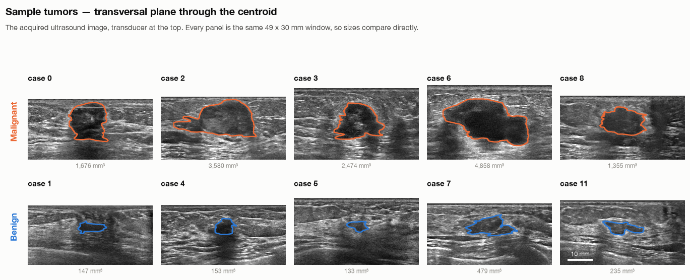
<p>The image below is one transversal slice through an ABUS volume from the TDSC-ABUS dataset this project uses — the same kind of slice a radiologist would scroll through, at a physical millimetre scale rather than raw pixels (ABUS voxels are not cubes, which turns out to matter a lot once you start measuring shape — more on that in a later post).</p>

<p align="center">
    <img width="90%" src="/assets/images/posts/projects/abus-classification/sample-tumors-transversal.png" />
</p>
<p align="center"><em>Five malignant and five benign lesions from the TDSC-ABUS dataset, each shown in the transversal plane through its centre at a common millimetre scale.</em></p>

<p>The coronal plane — the one roughly parallel to the chest wall, which a handheld scan essentially never captures — turns out to be particularly informative for malignancy, since it’s the plane in which spiculation (cancer’s characteristic radiating, starburst pattern) is most visible. That’s a recurring theme in the next post: several of the strongest classical features for this problem only exist because ABUS gives you a plane handheld ultrasound doesn’t.</p>

<p>The other side of automating the acquisition is that reading a full 3D volume, slice by slice, takes a radiologist considerably longer than glancing at a couple of 2D frames — which is the actual motivation for this whole project. If the volume is standardized and complete, it becomes something a model can be trained on, not just something a person has to scroll through. That’s where the rest of this series goes: turning what a radiologist looks for in a volume like the one above — shape, margins, spiculation, texture — into features and models that can flag and classify a lesion automatically.</p>

<h1 id="references">References</h1>

<ol>
  <li>T. M. Kolb, J. Lichy, J. H. Newhouse. Comparison of the performance of screening mammography, physical examination, and breast US and evaluation of factors that influence them: an analysis of 27,825 patient evaluations. <em>Radiology</em> 225(1):165–175, 2002. <a href="https://doi.org/10.1148/radiol.2251011667">doi:10.1148/radiol.2251011667</a></li>
  <li>W.-H. Yuan, H.-C. Hsu, Y.-Y. Chen, C.-H. Wu. Supplemental breast cancer-screening ultrasonography in women with dense breasts: a systematic review and meta-analysis. <em>British Journal of Cancer</em> 123:673–688, 2020. <a href="https://doi.org/10.1038/s41416-020-0928-1">doi:10.1038/s41416-020-0928-1</a></li>
  <li>J. C. M. van Zelst, R. M. Mann. Automated three-dimensional breast US for screening: technique, artifacts, and lesion characterization. <em>RadioGraphics</em> 38(3):663–683, 2018. <a href="https://doi.org/10.1148/rg.2018170162">doi:10.1148/rg.2018170162</a></li>
  <li>R. F. Brem, L. Tabár, S. W. Duffy, et al. Assessing improvement in detection of breast cancer with three-dimensional automated breast US in women with dense breast tissue: the SomoInsight study. <em>Radiology</em> 274(3):663–673, 2015. <a href="https://doi.org/10.1148/radiol.14132832">doi:10.1148/radiol.14132832</a></li>
</ol>]]></content><author><name>Ali Naderi</name></author><category term="project" /><category term="abus-classification" /><category term="medical-imaging" /><category term="ultrasound" /><category term="mammography" /><category term="breast-cancer" /><summary type="html"><![CDATA[This is the first post of a series following abus-classification, a project classifying malignant and benign breast lesions in 3D automated breast ultrasound (ABUS). I’ll add one post per phase of the project — this one is background, with no results yet: what a breast tumor is, how it gets imaged, and why this project uses 3D ultrasound specifically. The next post covers the classical radiology features we reproduce as a baseline; the one after that covers the deep-learning approaches.]]></summary></entry><entry><title type="html">Smart Card: Building Your First Applet with jCardSim</title><link href="https://alinaderiparizi.com/blog/embeded/smart-card/2026/09/04/smart-card-dev.html" rel="alternate" type="text/html" title="Smart Card: Building Your First Applet with jCardSim" /><published>2026-09-04T04:20:01+00:00</published><updated>2026-09-04T04:20:01+00:00</updated><id>https://alinaderiparizi.com/blog/embeded/smart-card/2026/09/04/smart-card-dev</id><content type="html" xml:base="https://alinaderiparizi.com/blog/embeded/smart-card/2026/09/04/smart-card-dev.html"><![CDATA[<h1 id="0-recap-and-the-goal">0. Recap and the goal</h1>

<p>In the <a href="/blog/embeded/smart-card/2023/07/19/smart-card-intro.html">previous post</a> we talked about what smart cards are, how they work, and what an applet is in the Java Card world: a small, isolated program that runs inside the card’s secure microprocessor and talks to the outside world through APDU commands.</p>

<p>That post ended with a promise: it’s time to actually write one.</p>

<p>But I also want to be upfront about <em>why</em> I’m going down this path. The real target of this series is not “print hello world on a card.” It’s building a hardware security token, a smart card that can act as a <strong>FIDO/U2F security key</strong>. FIDO keys (like a YubiKey) are, under the hood, exactly this kind of device: a secure element running an applet that generates and stores key pairs, signs authentication challenges, and never lets the private key leave the chip. Java Card gives us the same building blocks: isolated applet execution, on-card cryptography, and a well-defined command/response protocol over APDUs.</p>

<p>Before we touch real hardware, cryptography, or the FIDO protocol though, we need to get comfortable with the basics: writing an applet, installing it, and exchanging APDUs with it. And we’re going to do all of that <strong>without a physical smart card or reader</strong>, using a simulator called jCardSim.</p>

<h1 id="1-why-simulate-the-card-first">1. Why simulate the card first</h1>

<p>Real Java Card smart cards are cheap, but the development loop around them is not fun:</p>

<ul>
  <li>You need a physical card, a compatible reader, and often a card that accepts your own applets (many bank/SIM cards are locked down).</li>
  <li>Every test cycle means: compile, convert to a <code class="language-plaintext highlighter-rouge">.cap</code> file, load it onto the card over a reader, run it, and if something’s wrong, erase and repeat.</li>
  <li>Debugging is close to impossible. There’s no breakpoint, no stack trace, just a status word telling you something went wrong.</li>
</ul>

<p>That’s a painful way to learn a new, restricted dialect of Java. This is exactly the gap <strong>jCardSim</strong> fills.</p>

<h1 id="2-what-is-jcardsim">2. What is jCardSim</h1>

<p><a href="https://github.com/licel/jcardsim">jCardSim</a> is an open source, pure-Java simulator for the Java Card runtime environment (JCRE). It implements enough of the Java Card API (<code class="language-plaintext highlighter-rouge">javacard.framework</code>, <code class="language-plaintext highlighter-rouge">javacard.security</code>, and friends) to load and run real applet code, the same <code class="language-plaintext highlighter-rouge">.class</code> files you’d eventually convert into a <code class="language-plaintext highlighter-rouge">.cap</code> file for a physical card, entirely inside a JVM on your laptop.</p>

<p>A few things that make it genuinely useful, not just a toy:</p>

<ul>
  <li><strong>No hardware required.</strong> You write an applet, install it into a simulated card object, and start sending it APDUs immediately.</li>
  <li><strong>It speaks the same language as <code class="language-plaintext highlighter-rouge">javax.smartcardio</code>.</strong> jCardSim exposes a <code class="language-plaintext highlighter-rouge">CardSimulator</code> that you drive with the standard Java smart card I/O API (<code class="language-plaintext highlighter-rouge">CommandAPDU</code> / <code class="language-plaintext highlighter-rouge">ResponseAPDU</code>), the exact same classes you’d use to talk to a real card through a PC/SC reader. That means code you write against the simulator is structurally the same code you’d use against real hardware later.</li>
  <li><strong>It’s fast enough for real unit testing.</strong> We used it on real projects to write automated tests for applet logic (state machines, PIN verification, data encoding) in a normal CI pipeline, no reader, no lab, no flaky USB drivers.</li>
  <li><strong>It’s a stepping stone, not a replacement.</strong> The simulator doesn’t emulate every timing quirk or memory constraint of a real chip, so the last mile of testing on actual hardware still matters. But it removes 90% of the friction from the early development loop.</li>
</ul>

<p>For prototyping something like a FIDO applet, where you’ll be iterating a lot on command parsing, state handling, and cryptographic flows, this is exactly the tool you want before you ever plug in a real card.</p>

<h1 id="3-setting-up-the-project">3. Setting up the project</h1>

<p>A minimal Java Card + jCardSim project needs two sets of dependencies:</p>

<ol>
  <li>The <strong>Java Card Classic API</strong> (<code class="language-plaintext highlighter-rouge">javacard.framework</code>, etc.), just to compile against the applet interfaces. jCardSim ships an implementation of these on the classpath, so for a simulation-only project you don’t need Oracle/Global Platform’s official Java Card Development Kit at all.</li>
  <li><strong>jCardSim</strong> itself, to get <code class="language-plaintext highlighter-rouge">CardSimulator</code>, <code class="language-plaintext highlighter-rouge">AIDUtil</code>, and the simulated runtime classes.</li>
</ol>

<p>With Maven, a <code class="language-plaintext highlighter-rouge">pom.xml</code> for a small sandbox project looks roughly like this:</p>

<div class="language-xml highlighter-rouge"><div class="highlight"><pre class="highlight"><code><span class="nt">&lt;dependencies&gt;</span>
    <span class="nt">&lt;dependency&gt;</span>
        <span class="nt">&lt;groupId&gt;</span>com.licel<span class="nt">&lt;/groupId&gt;</span>
        <span class="nt">&lt;artifactId&gt;</span>jcardsim<span class="nt">&lt;/artifactId&gt;</span>
        <span class="nt">&lt;version&gt;</span>3.0.5-SNAPSHOT<span class="nt">&lt;/version&gt;</span>
    <span class="nt">&lt;/dependency&gt;</span>
<span class="nt">&lt;/dependencies&gt;</span>
</code></pre></div></div>

<p>The exact coordinates and available versions have moved around over the years (the project isn’t always on Maven Central), so if that dependency doesn’t resolve, grab the jar directly from the <a href="https://github.com/licel/jcardsim">jCardSim GitHub releases</a> or build it from source with the repo’s own instructions, and install it into your local <code class="language-plaintext highlighter-rouge">.m2</code> repository. Either way, once the jar is on your classpath you’re ready to write the applet itself.</p>

<h1 id="4-our-first-applet-generate-a-key-pair-and-sign-a-challenge">4. Our first applet: generate a key pair and sign a challenge</h1>

<p>A “Hello World” applet wouldn’t really tell us anything about the road ahead, so let’s skip straight to the thing a security key actually does: <strong>generate a key pair on the card, keep the private key locked inside it forever, and sign whatever challenge it’s asked to sign.</strong> That’s the entire trust model behind FIDO/U2F, register a public key once, then prove possession of the matching private key on every login, and it’s a handful of calls into <code class="language-plaintext highlighter-rouge">javacard.security</code>.</p>

<p>Every Java Card applet has the same shape: an <code class="language-plaintext highlighter-rouge">install()</code> factory method the JCRE calls when the applet is loaded, and a <code class="language-plaintext highlighter-rouge">process()</code> method the JCRE calls for every APDU sent to it. Ours generates its key pair once, at install time, and exposes two instructions: one to read back the public key, one to sign a challenge with the private key.</p>

<div class="language-java highlighter-rouge"><div class="highlight"><pre class="highlight"><code><span class="kn">package</span> <span class="nn">com.mralinp.simplesign</span><span class="o">;</span>

<span class="kn">import</span> <span class="nn">javacard.framework.APDU</span><span class="o">;</span>
<span class="kn">import</span> <span class="nn">javacard.framework.Applet</span><span class="o">;</span>
<span class="kn">import</span> <span class="nn">javacard.framework.ISO7816</span><span class="o">;</span>
<span class="kn">import</span> <span class="nn">javacard.framework.ISOException</span><span class="o">;</span>
<span class="kn">import</span> <span class="nn">javacard.security.KeyBuilder</span><span class="o">;</span>
<span class="kn">import</span> <span class="nn">javacard.security.KeyPair</span><span class="o">;</span>
<span class="kn">import</span> <span class="nn">javacard.security.RSAPublicKey</span><span class="o">;</span>
<span class="kn">import</span> <span class="nn">javacard.security.Signature</span><span class="o">;</span>

<span class="kd">public</span> <span class="kd">class</span> <span class="nc">SimpleSignApplet</span> <span class="kd">extends</span> <span class="nc">Applet</span> <span class="o">{</span>

    <span class="kd">private</span> <span class="kd">static</span> <span class="kd">final</span> <span class="kt">byte</span> <span class="no">INS_SIGN</span> <span class="o">=</span> <span class="o">(</span><span class="kt">byte</span><span class="o">)</span> <span class="mh">0x01</span><span class="o">;</span>
    <span class="kd">private</span> <span class="kd">static</span> <span class="kd">final</span> <span class="kt">byte</span> <span class="no">INS_GET_PUBLIC_KEY</span> <span class="o">=</span> <span class="o">(</span><span class="kt">byte</span><span class="o">)</span> <span class="mh">0x02</span><span class="o">;</span>

    <span class="kd">private</span> <span class="kd">final</span> <span class="nc">KeyPair</span> <span class="n">keyPair</span><span class="o">;</span>
    <span class="kd">private</span> <span class="kd">final</span> <span class="nc">Signature</span> <span class="n">signer</span><span class="o">;</span>

    <span class="kd">protected</span> <span class="nf">SimpleSignApplet</span><span class="o">()</span> <span class="o">{</span>
        <span class="c1">// Generate a fresh 1024-bit RSA key pair the moment the applet is installed.</span>
        <span class="c1">// The private key never leaves this object, and never leaves the card.</span>
        <span class="n">keyPair</span> <span class="o">=</span> <span class="k">new</span> <span class="nc">KeyPair</span><span class="o">(</span><span class="nc">KeyPair</span><span class="o">.</span><span class="na">ALG_RSA_CRT</span><span class="o">,</span> <span class="nc">KeyBuilder</span><span class="o">.</span><span class="na">LENGTH_RSA_1024</span><span class="o">);</span>
        <span class="n">keyPair</span><span class="o">.</span><span class="na">genKeyPair</span><span class="o">();</span>

        <span class="n">signer</span> <span class="o">=</span> <span class="nc">Signature</span><span class="o">.</span><span class="na">getInstance</span><span class="o">(</span><span class="nc">Signature</span><span class="o">.</span><span class="na">ALG_RSA_SHA_PKCS1</span><span class="o">,</span> <span class="kc">false</span><span class="o">);</span>
        <span class="n">register</span><span class="o">();</span>
    <span class="o">}</span>

    <span class="kd">public</span> <span class="kd">static</span> <span class="kt">void</span> <span class="nf">install</span><span class="o">(</span><span class="kt">byte</span><span class="o">[]</span> <span class="n">bArray</span><span class="o">,</span> <span class="kt">short</span> <span class="n">bOffset</span><span class="o">,</span> <span class="kt">byte</span> <span class="n">bLength</span><span class="o">)</span> <span class="o">{</span>
        <span class="k">new</span> <span class="nf">SimpleSignApplet</span><span class="o">();</span>
    <span class="o">}</span>

    <span class="nd">@Override</span>
    <span class="kd">public</span> <span class="kt">void</span> <span class="nf">process</span><span class="o">(</span><span class="no">APDU</span> <span class="n">apdu</span><span class="o">)</span> <span class="o">{</span>
        <span class="k">if</span> <span class="o">(</span><span class="n">selectingApplet</span><span class="o">())</span> <span class="o">{</span>
            <span class="k">return</span><span class="o">;</span>
        <span class="o">}</span>

        <span class="kt">byte</span><span class="o">[]</span> <span class="n">buffer</span> <span class="o">=</span> <span class="n">apdu</span><span class="o">.</span><span class="na">getBuffer</span><span class="o">();</span>
        <span class="kt">byte</span> <span class="n">instruction</span> <span class="o">=</span> <span class="n">buffer</span><span class="o">[</span><span class="no">ISO7816</span><span class="o">.</span><span class="na">OFFSET_INS</span><span class="o">];</span>

        <span class="k">switch</span> <span class="o">(</span><span class="n">instruction</span><span class="o">)</span> <span class="o">{</span>
            <span class="k">case</span> <span class="nl">INS_GET_PUBLIC_KEY:</span>
                <span class="n">sendPublicKey</span><span class="o">(</span><span class="n">apdu</span><span class="o">);</span>
                <span class="k">break</span><span class="o">;</span>
            <span class="k">case</span> <span class="nl">INS_SIGN:</span>
                <span class="n">signChallenge</span><span class="o">(</span><span class="n">apdu</span><span class="o">);</span>
                <span class="k">break</span><span class="o">;</span>
            <span class="k">default</span><span class="o">:</span>
                <span class="nc">ISOException</span><span class="o">.</span><span class="na">throwIt</span><span class="o">(</span><span class="no">ISO7816</span><span class="o">.</span><span class="na">SW_INS_NOT_SUPPORTED</span><span class="o">);</span>
        <span class="o">}</span>
    <span class="o">}</span>

    <span class="kd">private</span> <span class="kt">void</span> <span class="nf">sendPublicKey</span><span class="o">(</span><span class="no">APDU</span> <span class="n">apdu</span><span class="o">)</span> <span class="o">{</span>
        <span class="kt">byte</span><span class="o">[]</span> <span class="n">buffer</span> <span class="o">=</span> <span class="n">apdu</span><span class="o">.</span><span class="na">getBuffer</span><span class="o">();</span>
        <span class="nc">RSAPublicKey</span> <span class="n">publicKey</span> <span class="o">=</span> <span class="o">(</span><span class="nc">RSAPublicKey</span><span class="o">)</span> <span class="n">keyPair</span><span class="o">.</span><span class="na">getPublic</span><span class="o">();</span>

        <span class="c1">// buffer[0] holds the exponent length, so the caller knows where the modulus starts.</span>
        <span class="kt">short</span> <span class="n">exponentLength</span> <span class="o">=</span> <span class="n">publicKey</span><span class="o">.</span><span class="na">getExponent</span><span class="o">(</span><span class="n">buffer</span><span class="o">,</span> <span class="o">(</span><span class="kt">short</span><span class="o">)</span> <span class="mi">1</span><span class="o">);</span>
        <span class="n">buffer</span><span class="o">[</span><span class="mi">0</span><span class="o">]</span> <span class="o">=</span> <span class="o">(</span><span class="kt">byte</span><span class="o">)</span> <span class="n">exponentLength</span><span class="o">;</span>
        <span class="kt">short</span> <span class="n">modulusLength</span> <span class="o">=</span> <span class="n">publicKey</span><span class="o">.</span><span class="na">getModulus</span><span class="o">(</span><span class="n">buffer</span><span class="o">,</span> <span class="o">(</span><span class="kt">short</span><span class="o">)</span> <span class="o">(</span><span class="mi">1</span> <span class="o">+</span> <span class="n">exponentLength</span><span class="o">));</span>

        <span class="n">apdu</span><span class="o">.</span><span class="na">setOutgoingAndSend</span><span class="o">((</span><span class="kt">short</span><span class="o">)</span> <span class="mi">0</span><span class="o">,</span> <span class="o">(</span><span class="kt">short</span><span class="o">)</span> <span class="o">(</span><span class="mi">1</span> <span class="o">+</span> <span class="n">exponentLength</span> <span class="o">+</span> <span class="n">modulusLength</span><span class="o">));</span>
    <span class="o">}</span>

    <span class="kd">private</span> <span class="kt">void</span> <span class="nf">signChallenge</span><span class="o">(</span><span class="no">APDU</span> <span class="n">apdu</span><span class="o">)</span> <span class="o">{</span>
        <span class="kt">byte</span><span class="o">[]</span> <span class="n">buffer</span> <span class="o">=</span> <span class="n">apdu</span><span class="o">.</span><span class="na">getBuffer</span><span class="o">();</span>
        <span class="n">apdu</span><span class="o">.</span><span class="na">setIncomingAndReceive</span><span class="o">();</span>
        <span class="kt">short</span> <span class="n">challengeLength</span> <span class="o">=</span> <span class="n">apdu</span><span class="o">.</span><span class="na">getIncomingLength</span><span class="o">();</span>

        <span class="n">signer</span><span class="o">.</span><span class="na">init</span><span class="o">(</span><span class="n">keyPair</span><span class="o">.</span><span class="na">getPrivate</span><span class="o">(),</span> <span class="nc">Signature</span><span class="o">.</span><span class="na">MODE_SIGN</span><span class="o">);</span>
        <span class="kt">short</span> <span class="n">signatureLength</span> <span class="o">=</span> <span class="n">signer</span><span class="o">.</span><span class="na">sign</span><span class="o">(</span><span class="n">buffer</span><span class="o">,</span> <span class="no">ISO7816</span><span class="o">.</span><span class="na">OFFSET_CDATA</span><span class="o">,</span> <span class="n">challengeLength</span><span class="o">,</span> <span class="n">buffer</span><span class="o">,</span> <span class="o">(</span><span class="kt">short</span><span class="o">)</span> <span class="mi">0</span><span class="o">);</span>

        <span class="n">apdu</span><span class="o">.</span><span class="na">setOutgoingAndSend</span><span class="o">((</span><span class="kt">short</span><span class="o">)</span> <span class="mi">0</span><span class="o">,</span> <span class="n">signatureLength</span><span class="o">);</span>
    <span class="o">}</span>
<span class="o">}</span>
</code></pre></div></div>

<p>A couple of things worth calling out for anyone new to this API, since it looks like Java but behaves like embedded C in places:</p>

<ul>
  <li><code class="language-plaintext highlighter-rouge">install()</code> is a <strong>static factory</strong>, not a constructor you call yourself. The JCRE invokes it when the applet is loaded onto the card, and it’s responsible for constructing the applet instance and calling <code class="language-plaintext highlighter-rouge">register()</code> so the card knows this applet exists and can be selected. Key generation happens right there, once, up front, exactly the way a real token generates its device key the moment it’s provisioned.</li>
  <li><code class="language-plaintext highlighter-rouge">process()</code> is called for <strong>every single APDU</strong>, including the <code class="language-plaintext highlighter-rouge">SELECT</code> command used to activate the applet before anything else can happen. That’s why the very first thing we do is check <code class="language-plaintext highlighter-rouge">selectingApplet()</code> and return early, we don’t want to fall into our instruction switch for a <code class="language-plaintext highlighter-rouge">SELECT</code>.</li>
  <li>Everything happens through a <strong>shared APDU buffer</strong> (<code class="language-plaintext highlighter-rouge">apdu.getBuffer()</code>). There’s no heap of objects being passed around, incoming challenge bytes are read straight out of the buffer and the signature is written straight back into it. This is a direct consequence of how little RAM a real smart card chip has.</li>
  <li>The <code class="language-plaintext highlighter-rouge">RSAPrivateCrtKey</code> half of <code class="language-plaintext highlighter-rouge">keyPair</code> is never read, copied, or sent anywhere in this code. It only ever gets handed to <code class="language-plaintext highlighter-rouge">signer.init(...)</code>, which uses it internally to produce a signature. That’s the whole point: the card proves it holds the key without ever exposing it.</li>
</ul>

<p>We’re using RSA here rather than the ECDSA over P-256 that real FIDO devices use, mainly because RSA key generation needs nothing beyond a modulus length, while EC key generation on Java Card normally requires setting explicit curve domain parameters first. It keeps this first example short. When we build the real FIDO applet, we’ll switch <code class="language-plaintext highlighter-rouge">KeyPair.ALG_RSA_CRT</code> for <code class="language-plaintext highlighter-rouge">KeyPair.ALG_EC_FP</code> and set up the P-256 domain parameters properly.</p>

<h1 id="5-running-it-in-jcardsim">5. Running it in jCardSim</h1>

<p>Now the payoff: let’s install this applet into a simulated card, ask it for its public key, hand it a challenge to sign, and verify the signature ourselves, all without a physical card or reader.</p>

<div class="language-java highlighter-rouge"><div class="highlight"><pre class="highlight"><code><span class="kn">package</span> <span class="nn">com.mralinp.simplesign</span><span class="o">;</span>

<span class="kn">import</span> <span class="nn">com.licel.jcardsim.smartcardio.CardSimulator</span><span class="o">;</span>
<span class="kn">import</span> <span class="nn">com.licel.jcardsim.utils.AIDUtil</span><span class="o">;</span>
<span class="kn">import</span> <span class="nn">javacard.framework.AID</span><span class="o">;</span>

<span class="kn">import</span> <span class="nn">javax.smartcardio.CommandAPDU</span><span class="o">;</span>
<span class="kn">import</span> <span class="nn">javax.smartcardio.ResponseAPDU</span><span class="o">;</span>
<span class="kn">import</span> <span class="nn">java.math.BigInteger</span><span class="o">;</span>
<span class="kn">import</span> <span class="nn">java.security.KeyFactory</span><span class="o">;</span>
<span class="kn">import</span> <span class="nn">java.security.PublicKey</span><span class="o">;</span>
<span class="kn">import</span> <span class="nn">java.security.Signature</span><span class="o">;</span>
<span class="kn">import</span> <span class="nn">java.security.spec.RSAPublicKeySpec</span><span class="o">;</span>
<span class="kn">import</span> <span class="nn">java.util.Arrays</span><span class="o">;</span>

<span class="kd">public</span> <span class="kd">class</span> <span class="nc">SimpleSignTest</span> <span class="o">{</span>

    <span class="kd">public</span> <span class="kd">static</span> <span class="kt">void</span> <span class="nf">main</span><span class="o">(</span><span class="nc">String</span><span class="o">[]</span> <span class="n">args</span><span class="o">)</span> <span class="kd">throws</span> <span class="nc">Exception</span> <span class="o">{</span>
        <span class="c1">// 1. Create a simulated card and install our applet on it</span>
        <span class="nc">CardSimulator</span> <span class="n">simulator</span> <span class="o">=</span> <span class="k">new</span> <span class="nc">CardSimulator</span><span class="o">();</span>
        <span class="no">AID</span> <span class="n">appletAID</span> <span class="o">=</span> <span class="nc">AIDUtil</span><span class="o">.</span><span class="na">create</span><span class="o">(</span><span class="s">"A000000003000002"</span><span class="o">);</span>
        <span class="n">simulator</span><span class="o">.</span><span class="na">installApplet</span><span class="o">(</span><span class="n">appletAID</span><span class="o">,</span> <span class="nc">SimpleSignApplet</span><span class="o">.</span><span class="na">class</span><span class="o">);</span>
        <span class="n">simulator</span><span class="o">.</span><span class="na">selectApplet</span><span class="o">(</span><span class="n">appletAID</span><span class="o">);</span>

        <span class="c1">// 2. Ask the card for the public half of the key it generated at install time</span>
        <span class="nc">ResponseAPDU</span> <span class="n">pubKeyResponse</span> <span class="o">=</span> <span class="n">simulator</span><span class="o">.</span><span class="na">transmitCommand</span><span class="o">(</span><span class="k">new</span> <span class="nc">CommandAPDU</span><span class="o">(</span><span class="mh">0x00</span><span class="o">,</span> <span class="mh">0x02</span><span class="o">,</span> <span class="mh">0x00</span><span class="o">,</span> <span class="mh">0x00</span><span class="o">));</span>
        <span class="kt">byte</span><span class="o">[]</span> <span class="n">pubKeyBytes</span> <span class="o">=</span> <span class="n">pubKeyResponse</span><span class="o">.</span><span class="na">getData</span><span class="o">();</span>

        <span class="kt">int</span> <span class="n">exponentLength</span> <span class="o">=</span> <span class="n">pubKeyBytes</span><span class="o">[</span><span class="mi">0</span><span class="o">]</span> <span class="o">&amp;</span> <span class="mh">0xFF</span><span class="o">;</span>
        <span class="nc">BigInteger</span> <span class="n">exponent</span> <span class="o">=</span> <span class="k">new</span> <span class="nc">BigInteger</span><span class="o">(</span><span class="mi">1</span><span class="o">,</span> <span class="nc">Arrays</span><span class="o">.</span><span class="na">copyOfRange</span><span class="o">(</span><span class="n">pubKeyBytes</span><span class="o">,</span> <span class="mi">1</span><span class="o">,</span> <span class="mi">1</span> <span class="o">+</span> <span class="n">exponentLength</span><span class="o">));</span>
        <span class="nc">BigInteger</span> <span class="n">modulus</span> <span class="o">=</span> <span class="k">new</span> <span class="nc">BigInteger</span><span class="o">(</span><span class="mi">1</span><span class="o">,</span> <span class="nc">Arrays</span><span class="o">.</span><span class="na">copyOfRange</span><span class="o">(</span><span class="n">pubKeyBytes</span><span class="o">,</span> <span class="mi">1</span> <span class="o">+</span> <span class="n">exponentLength</span><span class="o">,</span> <span class="n">pubKeyBytes</span><span class="o">.</span><span class="na">length</span><span class="o">));</span>

        <span class="nc">PublicKey</span> <span class="n">publicKey</span> <span class="o">=</span> <span class="nc">KeyFactory</span><span class="o">.</span><span class="na">getInstance</span><span class="o">(</span><span class="s">"RSA"</span><span class="o">)</span>
                <span class="o">.</span><span class="na">generatePublic</span><span class="o">(</span><span class="k">new</span> <span class="nc">RSAPublicKeySpec</span><span class="o">(</span><span class="n">modulus</span><span class="o">,</span> <span class="n">exponent</span><span class="o">));</span>

        <span class="c1">// 3. Send a "login challenge" and have the card sign it with its private key</span>
        <span class="kt">byte</span><span class="o">[]</span> <span class="n">challenge</span> <span class="o">=</span> <span class="s">"login-challenge-42"</span><span class="o">.</span><span class="na">getBytes</span><span class="o">();</span>
        <span class="nc">ResponseAPDU</span> <span class="n">signResponse</span> <span class="o">=</span> <span class="n">simulator</span><span class="o">.</span><span class="na">transmitCommand</span><span class="o">(</span><span class="k">new</span> <span class="nc">CommandAPDU</span><span class="o">(</span><span class="mh">0x00</span><span class="o">,</span> <span class="mh">0x01</span><span class="o">,</span> <span class="mh">0x00</span><span class="o">,</span> <span class="mh">0x00</span><span class="o">,</span> <span class="n">challenge</span><span class="o">));</span>
        <span class="kt">byte</span><span class="o">[]</span> <span class="n">signature</span> <span class="o">=</span> <span class="n">signResponse</span><span class="o">.</span><span class="na">getData</span><span class="o">();</span>

        <span class="c1">// 4. Verify the signature ourselves, exactly like a server would on the other end</span>
        <span class="nc">Signature</span> <span class="n">verifier</span> <span class="o">=</span> <span class="nc">Signature</span><span class="o">.</span><span class="na">getInstance</span><span class="o">(</span><span class="s">"SHA1withRSA"</span><span class="o">);</span>
        <span class="n">verifier</span><span class="o">.</span><span class="na">initVerify</span><span class="o">(</span><span class="n">publicKey</span><span class="o">);</span>
        <span class="n">verifier</span><span class="o">.</span><span class="na">update</span><span class="o">(</span><span class="n">challenge</span><span class="o">);</span>

        <span class="nc">System</span><span class="o">.</span><span class="na">out</span><span class="o">.</span><span class="na">println</span><span class="o">(</span><span class="s">"Signature valid: "</span> <span class="o">+</span> <span class="n">verifier</span><span class="o">.</span><span class="na">verify</span><span class="o">(</span><span class="n">signature</span><span class="o">));</span>
    <span class="o">}</span>
<span class="o">}</span>
</code></pre></div></div>

<p>Running it prints:</p>

<div class="language-text highlighter-rouge"><div class="highlight"><pre class="highlight"><code>Signature valid: true
</code></pre></div></div>

<p>Nothing about steps 3 and 4 talked to the card, the private key stayed inside the simulated chip the entire time. We only ever handed the card a challenge and got a signature back, then verified that signature ourselves using nothing but the public key it gave us in step 2. That round trip, hand the token a challenge, get back a signature you can verify against a previously-registered public key, is the actual core of how a FIDO/U2F authentication works.</p>

<h1 id="6-where-this-is-going">6. Where this is going</h1>

<p>This applet is already doing the two things a real security key needs to do: keep a private key that never leaves the chip, and prove possession of it by signing on demand. What’s missing is the FIDO/U2F protocol wrapped around that behavior, a <code class="language-plaintext highlighter-rouge">REGISTER</code> command that returns a properly formatted attestation, an <code class="language-plaintext highlighter-rouge">AUTHENTICATE</code> command that tracks and increments a usage counter, ECDSA over the P-256 curve instead of RSA, and key handles instead of a single fixed key pair.</p>

<p>In the next post, we’ll build on this same jCardSim setup and start implementing the actual FIDO U2F command set on top of it, one instruction at a time, before ever touching a real card. Stay tuned.</p>

<h1 id="references">References</h1>

<ol>
  <li>Licel. jCardSim — Java Card simulator. GitHub. <a href="https://github.com/licel/jcardsim">github.com/licel/jcardsim</a></li>
  <li>Oracle. Java Card Classic Platform API Specification (<code class="language-plaintext highlighter-rouge">javacard.framework</code>, <code class="language-plaintext highlighter-rouge">javacard.security</code>). <a href="https://docs.oracle.com/javacard/">docs.oracle.com/javacard</a></li>
  <li>ISO/IEC 7816-4. Identification cards — Integrated circuit cards — Part 4: Organization, security and commands for interchange (APDU structure).</li>
  <li>FIDO Alliance. Universal 2nd Factor (U2F) Overview. <a href="https://fidoalliance.org/specs/u2f-specs-master/fido-u2f-overview.html">fidoalliance.org/specs/u2f-specs-master/fido-u2f-overview.html</a></li>
</ol>]]></content><author><name>Ali Naderi</name></author><category term="blog" /><category term="embeded" /><category term="smart-card" /><summary type="html"><![CDATA[0. Recap and the goal]]></summary></entry><entry><title type="html">Smart Card: An Introduction to smart card development</title><link href="https://alinaderiparizi.com/blog/embeded/smart-card/2023/07/19/smart-card-intro.html" rel="alternate" type="text/html" title="Smart Card: An Introduction to smart card development" /><published>2023-07-19T17:20:01+00:00</published><updated>2023-07-19T17:20:01+00:00</updated><id>https://alinaderiparizi.com/blog/embeded/smart-card/2023/07/19/smart-card-intro</id><content type="html" xml:base="https://alinaderiparizi.com/blog/embeded/smart-card/2023/07/19/smart-card-intro.html"><![CDATA[<h1 id="0-introduction">0. Introduction</h1>

<p>Smart cards are small, pocket-sized cards that contain an embedded microprocessor and memory chip. These cards are often made of plastic, and they look similar to traditional credit or debit cards, but they possess advanced technology that sets them apart. Smart cards are designed to securely store and process data, making them a powerful tool for various applications in today’s digital world.</p>

<p>There are two main types of smart cards:</p>

<ul>
  <li>
    <p><strong>Contact Smart Cards</strong>: These cards have gold-plated contact pads on their surface, which need to physically touch a card reader to establish communication. When inserted into a card reader or terminal, the contacts establish an electrical connection, enabling data transfer between the card and the reader. The data exchange can involve tasks such as authentication, data storage, and cryptographic operations.</p>
  </li>
  <li>
    <p><strong>Contactless Smart Cards</strong>: In contrast to contact smart cards, contactless smart cards do not require physical contact with a card reader. Instead, they use radio frequency identification (RFID) technology to communicate wirelessly with compatible card readers or terminals. This communication occurs when the card is placed within close proximity to the reader, making contactless smart cards particularly convenient and efficient for quick transactions.</p>
  </li>
</ul>

<p>Smart cards find applications in a wide range of industries and use cases, including:</p>

<ul>
  <li><strong>Financial Transactions</strong>: They are commonly used for secure payments in credit/debit cards, prepaid cards, and electronic wallets.</li>
  <li><strong>Access Control and Security</strong>: Smart cards are used for secure building access, network authentication, and data protection.</li>
  <li><strong>Healthcare</strong>: They facilitate secure access to electronic health records, patient identification, and prescription management.</li>
  <li><strong>Transportation</strong>: Smart cards are utilized in fare collection systems for public transport, allowing for seamless ticketing and fare management.</li>
  <li><strong>Government Identification</strong>: National ID cards, driver’s licenses, and electronic passports often incorporate smart card technology for enhanced security features.</li>
</ul>

<p>The ability of smart cards to securely store sensitive data, perform cryptographic operations, and communicate with various systems has made them an indispensable component of modern technology, ensuring safer and more efficient transactions and interactions in numerous domains.</p>

<p>Smart cards are equipped with a microprocessor and a specialized operating system, which sets them apart from traditional magnetic stripe cards. The presence of these components enables smart cards to perform more sophisticated functions and offer enhanced security features.</p>

<ol>
  <li>
    <p><strong>Microprocessor</strong>:
The microprocessor is the brain of the smart card, responsible for executing commands and processing data. It is a small integrated circuit that can perform complex calculations and cryptographic operations. The microprocessor allows the card to interact intelligently with card readers or terminals, enabling secure data exchange and executing specific tasks according to the applications it supports.</p>
  </li>
  <li>
    <p><strong>Operating System</strong>:
The operating system (OS) of a smart card is a specialized software that manages the card’s functions, controls access to its resources, and provides a standardized interface for applications to interact with the card’s hardware and data. The operating system facilitates communication with the outside world, ensuring that commands and data sent to the card are processed correctly and securely.</p>
  </li>
</ol>

<p>The presence of a microprocessor and an operating system on smart cards allows for several important capabilities:</p>

<ol>
  <li>
    <p><strong>Security Features</strong>:
Smart cards use their microprocessors to perform encryption and decryption operations, making them highly secure for sensitive transactions and data storage. The operating system plays a crucial role in managing cryptographic keys and ensuring secure access to the card’s data.</p>
  </li>
  <li>
    <p><strong>Secure Application Execution</strong>:
The operating system provides a secure environment for applications running on the smart card. It isolates different applications from one another, preventing unauthorized access and ensuring that one application’s activities cannot compromise the security of others on the same card.</p>
  </li>
  <li>
    <p><strong>Multiple Applications</strong>:
Smart cards have the ability to support multiple applications simultaneously. For example, a single smart card can be used for electronic payments, access control, and healthcare records. The operating system facilitates seamless execution and switching between these applications.</p>
  </li>
  <li>
    <p><strong>Dynamic Updates</strong>:
The operating system can be updated or patched to address security vulnerabilities or add new features to the smart card without replacing the physical card itself.</p>
  </li>
</ol>

<p>Due to these advanced features, smart cards have become a reliable and secure tool for various applications, such as financial transactions, secure access control, healthcare, and more. The combination of a microprocessor and an operating system empowers smart cards to deliver enhanced functionality, robust security, and unparalleled convenience in the digital age.</p>

<p>In the context of smart cards, an applet refers to a small, specialized software application that runs on the smart card’s microprocessor and is managed by the card’s operating system. These applets are designed to perform specific functions or provide particular services on the smart card. They enable the smart card to support various applications and perform tasks relevant to the cardholder’s needs.</p>

<h1 id="1-applets">1. Applets</h1>

<p>Applets on smart cards are comparable to apps on a smartphone. Each applet functions as a self-contained program with a defined set of functionalities, and multiple applets can coexist on the same smart card without interfering with each other. This modularity and isolation of applets are essential for maintaining security and ensuring that sensitive data from one application remains isolated from others.</p>

<p>The key characteristics of applets on smart cards include:</p>

<ol>
  <li>
    <p><strong>Security</strong>:
Applets are designed with security in mind, ensuring that the data and operations they perform remain protected from unauthorized access. The smart card’s operating system enforces strict access controls to prevent unauthorized applets from interfering with sensitive data or executing malicious operations.</p>
  </li>
  <li>
    <p><strong>Isolation</strong>:
Each applet runs within its own secure execution environment, isolated from other applets on the smart card. This isolation prevents one applet from accessing data or resources belonging to another, ensuring a high level of data privacy and integrity.</p>
  </li>
  <li>
    <p><strong>Flexibility</strong>:
Applets can be added, removed, or updated on the smart card without replacing the physical card itself. This flexibility allows card issuers to introduce new services or applications to the card without disrupting existing functionalities.</p>
  </li>
  <li>
    <p><strong>Common Criteria Compliance</strong>:
Applets are typically developed following the Common Criteria standard, which defines security requirements for evaluating and certifying the security of IT products, including smart cards.</p>
  </li>
</ol>

<p>Examples of applets on smart cards include:</p>

<ul>
  <li><strong>Payment Applet</strong>: Enables secure financial transactions and management of funds on the smart card, allowing it to be used as a debit or credit card.</li>
  <li><strong>Identity Applet</strong>: Stores and manages personal identification information for government-issued identification cards or electronic passports.</li>
  <li><strong>Health Applet</strong>: Manages electronic health records and provides secure access to patient information for healthcare applications.</li>
  <li><strong>Access Control Applet</strong>: Facilitates secure access to buildings, computer systems, or networks by providing authentication and authorization services.</li>
</ul>

<p>Overall, applets on smart cards play a crucial role in extending the card’s capabilities, enhancing security, and enabling multiple applications to coexist on a single card while maintaining data privacy and integrity.</p>

<h1 id="2-developing-applets">2. Developing Applets</h1>

<p>Writing applets for smart cards requires specialized skills and knowledge of smart card technology, microcontroller programming, and the specific programming language supported by the smart card’s microprocessor. Most smart cards use the Java Card platform, which allows developers to write applets in Java Card language.</p>

<p>Here are the general steps to write applets for smart cards:</p>

<ol>
  <li>
    <p><strong>Set Up Development Environment</strong>:
First, you need to set up the development environment for smart card applet development. This involves installing the necessary software development kit (SDK) provided by the smart card manufacturer or Java Card platform.</p>
  </li>
  <li>
    <p><strong>Learn Java Card Programming</strong>:
Familiarize yourself with Java Card programming, which is a subset of the Java programming language tailored for smart card development. Understand the limitations and specific features of Java Card, as it differs from regular Java programming.</p>
  </li>
  <li>
    <p><strong>Define Applet Functionality</strong>:
Determine the functionality you want your applet to provide. Identify the specific tasks the applet should perform on the smart card, such as handling financial transactions, managing access control, or storing and retrieving sensitive data.</p>
  </li>
  <li>
    <p><strong>Develop the Applet Code</strong>:
Write the applet code in Java Card language. This code will define the behavior and operations of the applet on the smart card. Ensure that the applet code adheres to the security requirements and best practices for smart card development.</p>
  </li>
  <li>
    <p><strong>Compile and Convert to CAP File</strong>:
After writing the applet code, compile it using the Java Card compiler to produce a .cap file (CAP stands for “Converted Applet”). This file contains the binary representation of the applet code, ready for installation on the smart card.</p>
  </li>
  <li>
    <p><strong>Load the Applet onto the Smart Card</strong>:
Use the appropriate tools or APIs provided by the smart card manufacturer or Java Card platform to load the .cap file onto the smart card. This process is known as “applet installation.”</p>
  </li>
  <li>
    <p><strong>Test and Debug</strong>:
Test the applet on the smart card to ensure that it functions as expected. Debug any issues that may arise during testing, making necessary adjustments to the applet code if needed.</p>
  </li>
  <li>
    <p><strong>Deploy and Distribute</strong>:
Once the applet is thoroughly tested and verified, it can be deployed on the desired smart cards or distributed to end-users through card issuers or service providers.</p>
  </li>
</ol>

<p>Please note that writing applets for smart cards requires expertise in smart card development and may vary depending on the specific smart card’s capabilities and the programming language supported by its microprocessor. It’s essential to refer to the smart card manufacturer’s documentation and Java Card specifications for detailed guidelines and best practices when developing applets for smart cards.</p>

<p>Next time, I’ll prepare an article about developing an applet and playing around with this old technology. Stay tuned…</p>

<h1 id="references">References</h1>

<ol>
  <li>ISO/IEC 7816 (all parts). Identification cards — Integrated circuit cards. International Organization for Standardization.</li>
  <li>GlobalPlatform. Card Specification. <a href="https://globalplatform.org/specs-library/">globalplatform.org/specs-library</a></li>
  <li>Oracle. Java Card Technology. <a href="https://www.oracle.com/java/technologies/java-card-tech.html">oracle.com/java/technologies/java-card-tech.html</a></li>
</ol>]]></content><author><name>Ali Naderi</name></author><category term="blog" /><category term="embeded" /><category term="smart-card" /><summary type="html"><![CDATA[0. Introduction]]></summary></entry><entry><title type="html">PyTorch Tutorial, Part 2: Datasets and DataLoaders</title><link href="https://alinaderiparizi.com/blog/ai/machine-learning/deep-learning/python/pytorch/2023/03/27/pytorch-tutorial-2.html" rel="alternate" type="text/html" title="PyTorch Tutorial, Part 2: Datasets and DataLoaders" /><published>2023-03-27T13:45:23+00:00</published><updated>2023-03-27T13:45:23+00:00</updated><id>https://alinaderiparizi.com/blog/ai/machine-learning/deep-learning/python/pytorch/2023/03/27/pytorch-tutorial-2</id><content type="html" xml:base="https://alinaderiparizi.com/blog/ai/machine-learning/deep-learning/python/pytorch/2023/03/27/pytorch-tutorial-2.html"><![CDATA[<p><a href="/blog/ai/machine-learning/deep-learning/python/pytorch/2023/03/22/pytorch-tutorial-1.html">Part 1</a> trained on data that lived entirely in a few lines of Python — five numbers, or a scikit-learn dataset that loads fully into memory in one call. Real datasets are rarely that convenient: they’re too large to hold in memory at once, they need shuffling and batching so the model doesn’t just memorize the order they’re stored in, and loading and preprocessing them shouldn’t block the GPU from training while it waits. PyTorch’s <code class="language-plaintext highlighter-rouge">Dataset</code> and <code class="language-plaintext highlighter-rouge">DataLoader</code> classes exist specifically to solve that, by cleanly separating two concerns that are easy to tangle together: <em>what</em> your data is and how to fetch one example of it (<code class="language-plaintext highlighter-rouge">Dataset</code>), and <em>how</em> to turn a stream of individual examples into shuffled, batched tensors ready for a training loop (<code class="language-plaintext highlighter-rouge">DataLoader</code>). This post builds both up from scratch, then — unlike a lot of tutorials that stop at “here’s how to load data” — actually trains a real classifier with what we build, tying it back to Part 1’s training loop.</p>

<h1 id="1-a-custom-dataset">1. A custom Dataset</h1>

<p>We’ll use the classic <a href="https://archive.ics.uci.edu/dataset/109/wine">Wine dataset</a> from the UCI Machine Learning Repository [1]: 178 wine samples, each with 13 chemical measurements (alcohol content, malic acid, ash, and so on) and a label — which of three cultivars the wine came from. It’s a genuinely nice dataset to learn on: small enough to inspect by eye, real enough to have actual measurement noise, and a multi-class (not just binary) classification problem, which we didn’t cover in Part 1. Download <code class="language-plaintext highlighter-rouge">wine.data</code> from the repository page and place it somewhere like <code class="language-plaintext highlighter-rouge">../data/wine/wine.data</code> relative to your script (I keep a <code class="language-plaintext highlighter-rouge">data/</code> directory alongside my code for exactly this).</p>

<p>Every PyTorch <code class="language-plaintext highlighter-rouge">Dataset</code> is a class inheriting from <code class="language-plaintext highlighter-rouge">torch.utils.data.Dataset</code> that implements exactly two methods: <code class="language-plaintext highlighter-rouge">__getitem__(self, index)</code>, returning the sample at that index, and <code class="language-plaintext highlighter-rouge">__len__(self)</code>, returning the total number of samples. That’s the entire contract — PyTorch doesn’t care <em>how</em> you fetch a sample (from a NumPy array already in memory, from a file you open lazily on each call, from a network request), only that these two methods work.</p>

<div class="language-python highlighter-rouge"><div class="highlight"><pre class="highlight"><code><span class="kn">import</span> <span class="nn">torch</span>
<span class="kn">import</span> <span class="nn">numpy</span> <span class="k">as</span> <span class="n">np</span>

<span class="n">PATH_TO_DATASET</span> <span class="o">=</span> <span class="s">'../data/wine/wine.data'</span>

<span class="k">class</span> <span class="nc">WineDataset</span><span class="p">(</span><span class="n">torch</span><span class="p">.</span><span class="n">utils</span><span class="p">.</span><span class="n">data</span><span class="p">.</span><span class="n">Dataset</span><span class="p">):</span>
    <span class="k">def</span> <span class="nf">__init__</span><span class="p">(</span><span class="bp">self</span><span class="p">)</span> <span class="o">-&gt;</span> <span class="bp">None</span><span class="p">:</span>
        <span class="c1"># The file is one row per sample, comma-separated, label in column 0
</span>        <span class="c1"># and the 13 features in the remaining columns.
</span>        <span class="n">raw_data</span> <span class="o">=</span> <span class="n">np</span><span class="p">.</span><span class="n">loadtxt</span><span class="p">(</span><span class="n">PATH_TO_DATASET</span><span class="p">,</span> <span class="n">delimiter</span><span class="o">=</span><span class="s">','</span><span class="p">,</span> <span class="n">dtype</span><span class="o">=</span><span class="n">np</span><span class="p">.</span><span class="n">float32</span><span class="p">)</span>
        <span class="bp">self</span><span class="p">.</span><span class="n">x</span> <span class="o">=</span> <span class="n">torch</span><span class="p">.</span><span class="n">from_numpy</span><span class="p">(</span><span class="n">raw_data</span><span class="p">[:,</span> <span class="mi">1</span><span class="p">:])</span>
        <span class="bp">self</span><span class="p">.</span><span class="n">y</span> <span class="o">=</span> <span class="n">torch</span><span class="p">.</span><span class="n">from_numpy</span><span class="p">(</span><span class="n">raw_data</span><span class="p">[:,</span> <span class="p">[</span><span class="mi">0</span><span class="p">]])</span>
        <span class="bp">self</span><span class="p">.</span><span class="n">n_samples</span> <span class="o">=</span> <span class="bp">self</span><span class="p">.</span><span class="n">x</span><span class="p">.</span><span class="n">shape</span><span class="p">[</span><span class="mi">0</span><span class="p">]</span>
        <span class="bp">self</span><span class="p">.</span><span class="n">n_features</span> <span class="o">=</span> <span class="bp">self</span><span class="p">.</span><span class="n">x</span><span class="p">.</span><span class="n">shape</span><span class="p">[</span><span class="mi">1</span><span class="p">]</span>

    <span class="k">def</span> <span class="nf">__getitem__</span><span class="p">(</span><span class="bp">self</span><span class="p">,</span> <span class="n">index</span><span class="p">):</span>
        <span class="k">return</span> <span class="bp">self</span><span class="p">.</span><span class="n">x</span><span class="p">[</span><span class="n">index</span><span class="p">],</span> <span class="bp">self</span><span class="p">.</span><span class="n">y</span><span class="p">[</span><span class="n">index</span><span class="p">]</span>

    <span class="k">def</span> <span class="nf">__len__</span><span class="p">(</span><span class="bp">self</span><span class="p">):</span>
        <span class="k">return</span> <span class="bp">self</span><span class="p">.</span><span class="n">n_samples</span>
</code></pre></div></div>

<p>Now we can use it like any indexable, sized Python object:</p>

<div class="language-python highlighter-rouge"><div class="highlight"><pre class="highlight"><code><span class="n">dataset</span> <span class="o">=</span> <span class="n">WineDataset</span><span class="p">()</span>
<span class="k">print</span><span class="p">(</span><span class="sa">f</span><span class="s">"</span><span class="si">{</span><span class="nb">len</span><span class="p">(</span><span class="n">dataset</span><span class="p">)</span><span class="si">}</span><span class="s"> samples, </span><span class="si">{</span><span class="n">dataset</span><span class="p">.</span><span class="n">n_features</span><span class="si">}</span><span class="s"> features each"</span><span class="p">)</span>
<span class="n">x_sample</span><span class="p">,</span> <span class="n">y_sample</span> <span class="o">=</span> <span class="n">dataset</span><span class="p">[</span><span class="mi">0</span><span class="p">]</span>
<span class="k">print</span><span class="p">(</span><span class="sa">f</span><span class="s">"x: </span><span class="si">{</span><span class="n">x_sample</span><span class="si">}</span><span class="s">, y: </span><span class="si">{</span><span class="n">y_sample</span><span class="si">}</span><span class="s">"</span><span class="p">)</span>
</code></pre></div></div>

<pre><code class="language-txt">178 samples, 13 features each
x: tensor([1.4230e+01, 1.7100e+00, 2.4300e+00, 1.5600e+01, 1.2700e+02, 2.8000e+00,
        3.0600e+00, 2.8000e-01, 2.2900e+00, 5.6400e+00, 1.0400e+00, 3.9200e+00,
        1.0650e+03]), y: tensor([1.])
</code></pre>

<p><strong>If you’d rather skip the manual download</strong> while learning, scikit-learn ships this exact dataset built in — <code class="language-plaintext highlighter-rouge">sklearn.datasets.load_wine()</code> returns the same 178-sample, 13-feature data without touching the filesystem. Either source is fine for this post; we’ll stick with the custom-file version above because loading your <em>own</em> CSV or data file, not a bundled toy dataset, is the far more common real-world need this section is actually teaching.</p>

<p>That’s it — it looks almost too simple, and that’s the point. The class does nothing exotic; it just gives PyTorch a uniform interface so everything downstream (batching, shuffling, parallel loading) can be written once, generically, for <em>any</em> dataset that implements these two methods.</p>

<h1 id="2-dataloader">2. DataLoader</h1>

<p>A <code class="language-plaintext highlighter-rouge">Dataset</code> alone only gets you one sample at a time. <code class="language-plaintext highlighter-rouge">torch.utils.data.DataLoader</code> wraps a <code class="language-plaintext highlighter-rouge">Dataset</code> and handles everything you actually want during training: grouping samples into batches, shuffling their order every epoch, and optionally loading them in parallel.</p>

<div class="language-python highlighter-rouge"><div class="highlight"><pre class="highlight"><code><span class="n">dataloader</span> <span class="o">=</span> <span class="n">torch</span><span class="p">.</span><span class="n">utils</span><span class="p">.</span><span class="n">data</span><span class="p">.</span><span class="n">DataLoader</span><span class="p">(</span><span class="n">dataset</span><span class="o">=</span><span class="n">dataset</span><span class="p">,</span> <span class="n">batch_size</span><span class="o">=</span><span class="mi">16</span><span class="p">,</span> <span class="n">shuffle</span><span class="o">=</span><span class="bp">True</span><span class="p">,</span> <span class="n">num_workers</span><span class="o">=</span><span class="mi">2</span><span class="p">)</span>
</code></pre></div></div>

<p>Each argument is doing a specific, named job worth understanding rather than copy-pasting:</p>

<ul>
  <li><strong><code class="language-plaintext highlighter-rouge">batch_size</code></strong> — how many samples to group into one tensor per training step. Training on one sample at a time is slow (poor use of GPU parallelism) and noisy (each update is based on very little information); training on the <em>entire</em> dataset at once (<code class="language-plaintext highlighter-rouge">batch_size = len(dataset)</code>) is the other extreme — one very stable but very infrequent and memory-hungry update per epoch. Something in between — commonly 16, 32, 64, … — is the usual sweet spot, and it’s a hyperparameter worth experimenting with rather than treating as fixed.</li>
  <li><strong><code class="language-plaintext highlighter-rouge">shuffle=True</code></strong> — reshuffles the dataset’s order at the start of every epoch. Without this, a model can pick up on spurious patterns tied to <em>storage order</em> (e.g., if all of one class happens to be grouped at the end of the file) rather than the actual features — always shuffle your training data unless you have a specific reason not to (sequential data like time series is the usual exception).</li>
  <li><strong><code class="language-plaintext highlighter-rouge">num_workers</code></strong> — how many separate OS processes load and preprocess batches in the background, in parallel with the GPU training on the <em>previous</em> batch, so the GPU spends less time idle waiting for data. <code class="language-plaintext highlighter-rouge">0</code> (the default) loads data in the main process, which is simplest and fine for small in-memory datasets like this one; it starts mattering once loading involves real work (decoding images, reading from disk). One Windows/macOS-specific gotcha: with <code class="language-plaintext highlighter-rouge">num_workers &gt; 0</code>, your training script needs its DataLoader-using code inside an <code class="language-plaintext highlighter-rouge">if __name__ == '__main__':</code> guard, because those platforms re-import your script in each worker process, and without the guard you get infinite recursive process spawning.</li>
</ul>

<p>You can iterate a <code class="language-plaintext highlighter-rouge">DataLoader</code> directly, and it hands you one batch at a time:</p>

<div class="language-python highlighter-rouge"><div class="highlight"><pre class="highlight"><code><span class="k">for</span> <span class="n">batch_x</span><span class="p">,</span> <span class="n">batch_y</span> <span class="ow">in</span> <span class="n">dataloader</span><span class="p">:</span>
    <span class="k">print</span><span class="p">(</span><span class="n">batch_x</span><span class="p">.</span><span class="n">shape</span><span class="p">,</span> <span class="n">batch_y</span><span class="p">.</span><span class="n">shape</span><span class="p">)</span>   <span class="c1"># torch.Size([16, 13]) torch.Size([16, 1])
</span>    <span class="k">break</span>  <span class="c1"># just peek at the first batch
</span></code></pre></div></div>

<p>Or, if you want a single batch without a loop (useful for quick inspection in a notebook), wrap it in <code class="language-plaintext highlighter-rouge">iter()</code> and call <code class="language-plaintext highlighter-rouge">next()</code>:</p>

<div class="language-python highlighter-rouge"><div class="highlight"><pre class="highlight"><code><span class="n">dataiter</span> <span class="o">=</span> <span class="nb">iter</span><span class="p">(</span><span class="n">dataloader</span><span class="p">)</span>
<span class="n">x</span><span class="p">,</span> <span class="n">y</span> <span class="o">=</span> <span class="nb">next</span><span class="p">(</span><span class="n">dataiter</span><span class="p">)</span>
<span class="k">print</span><span class="p">(</span><span class="n">x</span><span class="p">,</span> <span class="n">y</span><span class="p">)</span>
</code></pre></div></div>

<pre><code class="language-txt">tensor([[1.3740e+01, 1.6700e+00, 2.2500e+00,  ..., 9.2000e-01, 3.2000e+00, 1.0600e+03],
        [1.1660e+01, 1.8800e+00, 1.9200e+00,  ..., 1.2300e+00, 2.1400e+00, 4.2800e+02],
        ...
        [1.3500e+01, 1.8100e+00, 2.6100e+00,  ..., ...              ]])
tensor([[1.], [2.], [1.], ...])
</code></pre>

<p>In real training loops you’ll almost always use the <code class="language-plaintext highlighter-rouge">for batch_x, batch_y in dataloader:</code> form directly (we’ll do exactly that in Section 4) — <code class="language-plaintext highlighter-rouge">iter()</code>/<code class="language-plaintext highlighter-rouge">next()</code> is mainly useful for debugging or peeking at a batch’s shape and content interactively.</p>

<h2 id="21-splitting-into-train-and-test-sets">2.1 Splitting into train and test sets</h2>

<p><code class="language-plaintext highlighter-rouge">WineDataset</code> above loads the whole file as one dataset, but we need separate train and test splits, the same way <code class="language-plaintext highlighter-rouge">train_test_split</code> did in Part 1. <code class="language-plaintext highlighter-rouge">torch.utils.data.random_split</code> does the same job directly on a <code class="language-plaintext highlighter-rouge">Dataset</code> object, without pulling everything into NumPy first:</p>

<div class="language-python highlighter-rouge"><div class="highlight"><pre class="highlight"><code><span class="n">train_size</span> <span class="o">=</span> <span class="nb">int</span><span class="p">(</span><span class="mf">0.8</span> <span class="o">*</span> <span class="nb">len</span><span class="p">(</span><span class="n">dataset</span><span class="p">))</span>
<span class="n">test_size</span> <span class="o">=</span> <span class="nb">len</span><span class="p">(</span><span class="n">dataset</span><span class="p">)</span> <span class="o">-</span> <span class="n">train_size</span>
<span class="n">train_dataset</span><span class="p">,</span> <span class="n">test_dataset</span> <span class="o">=</span> <span class="n">torch</span><span class="p">.</span><span class="n">utils</span><span class="p">.</span><span class="n">data</span><span class="p">.</span><span class="n">random_split</span><span class="p">(</span><span class="n">dataset</span><span class="p">,</span> <span class="p">[</span><span class="n">train_size</span><span class="p">,</span> <span class="n">test_size</span><span class="p">])</span>

<span class="n">train_loader</span> <span class="o">=</span> <span class="n">torch</span><span class="p">.</span><span class="n">utils</span><span class="p">.</span><span class="n">data</span><span class="p">.</span><span class="n">DataLoader</span><span class="p">(</span><span class="n">train_dataset</span><span class="p">,</span> <span class="n">batch_size</span><span class="o">=</span><span class="mi">16</span><span class="p">,</span> <span class="n">shuffle</span><span class="o">=</span><span class="bp">True</span><span class="p">)</span>
<span class="n">test_loader</span> <span class="o">=</span> <span class="n">torch</span><span class="p">.</span><span class="n">utils</span><span class="p">.</span><span class="n">data</span><span class="p">.</span><span class="n">DataLoader</span><span class="p">(</span><span class="n">test_dataset</span><span class="p">,</span> <span class="n">batch_size</span><span class="o">=</span><span class="mi">16</span><span class="p">,</span> <span class="n">shuffle</span><span class="o">=</span><span class="bp">False</span><span class="p">)</span>
</code></pre></div></div>

<p>Shuffling the test loader isn’t necessary (we’re not training on it, and order doesn’t affect evaluation), so it’s conventional to leave <code class="language-plaintext highlighter-rouge">shuffle=False</code> there — it’s one less source of non-determinism when you’re comparing runs.</p>

<h1 id="3-transforms">3. Transforms</h1>

<p>Sometimes you need to modify raw data before using it — normalizing values to a consistent scale (Part 1’s <code class="language-plaintext highlighter-rouge">StandardScaler</code> did this for the breast cancer features), converting types, or, for images specifically, data augmentation: randomly cropping, flipping, or color-jittering each image slightly differently on every epoch, so the model sees a slightly different version of the “same” example each time and generalizes better instead of memorizing exact pixels. We can support this in our own <code class="language-plaintext highlighter-rouge">Dataset</code> by accepting an optional list of transform functions in the constructor, and applying them in order inside <code class="language-plaintext highlighter-rouge">__getitem__</code>:</p>

<div class="language-python highlighter-rouge"><div class="highlight"><pre class="highlight"><code><span class="k">class</span> <span class="nc">WineDataset</span><span class="p">(</span><span class="n">torch</span><span class="p">.</span><span class="n">utils</span><span class="p">.</span><span class="n">data</span><span class="p">.</span><span class="n">Dataset</span><span class="p">):</span>

    <span class="k">def</span> <span class="nf">__init__</span><span class="p">(</span><span class="bp">self</span><span class="p">,</span> <span class="n">transforms</span><span class="o">=</span><span class="bp">None</span><span class="p">)</span> <span class="o">-&gt;</span> <span class="bp">None</span><span class="p">:</span>
        <span class="n">raw_data</span> <span class="o">=</span> <span class="n">np</span><span class="p">.</span><span class="n">loadtxt</span><span class="p">(</span><span class="n">PATH_TO_DATASET</span><span class="p">,</span> <span class="n">delimiter</span><span class="o">=</span><span class="s">','</span><span class="p">,</span> <span class="n">dtype</span><span class="o">=</span><span class="n">np</span><span class="p">.</span><span class="n">float32</span><span class="p">)</span>
        <span class="bp">self</span><span class="p">.</span><span class="n">x</span> <span class="o">=</span> <span class="n">raw_data</span><span class="p">[:,</span> <span class="mi">1</span><span class="p">:]</span>
        <span class="bp">self</span><span class="p">.</span><span class="n">y</span> <span class="o">=</span> <span class="n">raw_data</span><span class="p">[:,</span> <span class="p">[</span><span class="mi">0</span><span class="p">]]</span>
        <span class="bp">self</span><span class="p">.</span><span class="n">n_samples</span> <span class="o">=</span> <span class="bp">self</span><span class="p">.</span><span class="n">x</span><span class="p">.</span><span class="n">shape</span><span class="p">[</span><span class="mi">0</span><span class="p">]</span>
        <span class="bp">self</span><span class="p">.</span><span class="n">n_features</span> <span class="o">=</span> <span class="bp">self</span><span class="p">.</span><span class="n">x</span><span class="p">.</span><span class="n">shape</span><span class="p">[</span><span class="mi">1</span><span class="p">]</span>
        <span class="bp">self</span><span class="p">.</span><span class="n">transforms</span> <span class="o">=</span> <span class="n">transforms</span> <span class="ow">or</span> <span class="p">[]</span>

    <span class="k">def</span> <span class="nf">__getitem__</span><span class="p">(</span><span class="bp">self</span><span class="p">,</span> <span class="n">index</span><span class="p">):</span>
        <span class="n">sample</span> <span class="o">=</span> <span class="p">(</span><span class="bp">self</span><span class="p">.</span><span class="n">x</span><span class="p">[</span><span class="n">index</span><span class="p">],</span> <span class="bp">self</span><span class="p">.</span><span class="n">y</span><span class="p">[</span><span class="n">index</span><span class="p">])</span>
        <span class="k">for</span> <span class="n">transform</span> <span class="ow">in</span> <span class="bp">self</span><span class="p">.</span><span class="n">transforms</span><span class="p">:</span>
            <span class="n">sample</span> <span class="o">=</span> <span class="n">transform</span><span class="p">(</span><span class="n">sample</span><span class="p">)</span>
        <span class="k">return</span> <span class="n">sample</span>

    <span class="k">def</span> <span class="nf">__len__</span><span class="p">(</span><span class="bp">self</span><span class="p">):</span>
        <span class="k">return</span> <span class="bp">self</span><span class="p">.</span><span class="n">n_samples</span>
</code></pre></div></div>

<p>A transform can be any callable, but the idiomatic PyTorch pattern is a class implementing <code class="language-plaintext highlighter-rouge">__call__</code>, so a transform can carry its own configuration (like the scale factor below) as ordinary attributes:</p>

<div class="language-python highlighter-rouge"><div class="highlight"><pre class="highlight"><code><span class="k">class</span> <span class="nc">ToTensorTransformer</span><span class="p">:</span>
    <span class="k">def</span> <span class="nf">__call__</span><span class="p">(</span><span class="bp">self</span><span class="p">,</span> <span class="n">sample</span><span class="p">):</span>
        <span class="n">x</span><span class="p">,</span> <span class="n">y</span> <span class="o">=</span> <span class="n">sample</span>
        <span class="k">return</span> <span class="n">torch</span><span class="p">.</span><span class="n">from_numpy</span><span class="p">(</span><span class="n">x</span><span class="p">),</span> <span class="n">torch</span><span class="p">.</span><span class="n">from_numpy</span><span class="p">(</span><span class="n">y</span><span class="p">)</span>

<span class="k">class</span> <span class="nc">MultiplierTransformer</span><span class="p">:</span>

    <span class="k">def</span> <span class="nf">__init__</span><span class="p">(</span><span class="bp">self</span><span class="p">,</span> <span class="n">factor</span><span class="p">:</span> <span class="nb">float</span><span class="p">):</span>
        <span class="bp">self</span><span class="p">.</span><span class="n">factor</span> <span class="o">=</span> <span class="n">factor</span>

    <span class="k">def</span> <span class="nf">__call__</span><span class="p">(</span><span class="bp">self</span><span class="p">,</span> <span class="n">sample</span><span class="p">):</span>
        <span class="n">x</span><span class="p">,</span> <span class="n">y</span> <span class="o">=</span> <span class="n">sample</span>
        <span class="n">x</span> <span class="o">=</span> <span class="n">x</span> <span class="o">*</span> <span class="bp">self</span><span class="p">.</span><span class="n">factor</span>
        <span class="k">return</span> <span class="n">x</span><span class="p">,</span> <span class="n">y</span>
</code></pre></div></div>

<p>Pass a list of transforms to the constructor, and they’re applied in order, each one’s output feeding the next:</p>

<div class="language-python highlighter-rouge"><div class="highlight"><pre class="highlight"><code><span class="n">dataset</span> <span class="o">=</span> <span class="n">WineDataset</span><span class="p">(</span><span class="n">transforms</span><span class="o">=</span><span class="p">[</span><span class="n">ToTensorTransformer</span><span class="p">(),</span> <span class="n">MultiplierTransformer</span><span class="p">(</span><span class="mi">10</span><span class="p">)])</span>
<span class="n">x_sample</span><span class="p">,</span> <span class="n">y_sample</span> <span class="o">=</span> <span class="n">dataset</span><span class="p">[</span><span class="mi">0</span><span class="p">]</span>
<span class="k">print</span><span class="p">(</span><span class="sa">f</span><span class="s">"x: </span><span class="si">{</span><span class="n">x_sample</span><span class="si">}</span><span class="s">, y: </span><span class="si">{</span><span class="n">y_sample</span><span class="si">}</span><span class="s">"</span><span class="p">)</span>
</code></pre></div></div>

<pre><code class="language-txt">x: tensor([1.4230e+02, 1.7100e+01, 2.4300e+01, 1.5600e+02, 1.2700e+03, 2.8000e+01,
        3.0600e+01, 2.8000e+00, 2.2900e+01, 5.6400e+01, 1.0400e+01, 3.9200e+01,
        1.0650e+04]), y: tensor([1.])
</code></pre>

<p>This hand-rolled pattern is worth building once to understand it, but for real work — especially with images — reach for <code class="language-plaintext highlighter-rouge">torchvision.transforms.Compose</code> instead of writing your own list-and-loop logic: it’s the same idea (a sequence of callables, applied in order) with a large library of ready-made, well-tested transforms (resizing, cropping, normalization, augmentation) already implemented [2].</p>

<h1 id="4-putting-it-together-training-a-real-classifier">4. Putting it together: training a real classifier</h1>

<p>Everything so far has been plumbing. Let’s use it: a small neural network, trained on <code class="language-plaintext highlighter-rouge">WineDataset</code> through a <code class="language-plaintext highlighter-rouge">DataLoader</code>, classifying wine samples into one of three cultivars — combining this post’s data pipeline with Part 1’s training loop.</p>

<p>Two wrinkles specific to multi-class classification, worth flagging before the code: the Wine dataset’s labels are <code class="language-plaintext highlighter-rouge">1</code>, <code class="language-plaintext highlighter-rouge">2</code>, <code class="language-plaintext highlighter-rouge">3</code>, but PyTorch’s multi-class loss function expects <code class="language-plaintext highlighter-rouge">0</code>-indexed integer class labels, so we subtract 1; and instead of Part 1’s single output neuron plus sigmoid (built for <em>binary</em> classification — one probability), we now need <strong>one output per class</strong>, interpreted as that class’s un-normalized score, and PyTorch’s <code class="language-plaintext highlighter-rouge">CrossEntropyLoss</code> — which combines a softmax (turning raw scores into a probability distribution over classes) and negative-log-likelihood loss into one numerically stable operation — expects exactly that: raw scores in, integer class index out, no manual softmax needed.</p>

<div class="language-python highlighter-rouge"><div class="highlight"><pre class="highlight"><code><span class="kn">import</span> <span class="nn">torch</span>
<span class="kn">import</span> <span class="nn">numpy</span> <span class="k">as</span> <span class="n">np</span>

<span class="k">class</span> <span class="nc">WineDataset</span><span class="p">(</span><span class="n">torch</span><span class="p">.</span><span class="n">utils</span><span class="p">.</span><span class="n">data</span><span class="p">.</span><span class="n">Dataset</span><span class="p">):</span>
    <span class="k">def</span> <span class="nf">__init__</span><span class="p">(</span><span class="bp">self</span><span class="p">)</span> <span class="o">-&gt;</span> <span class="bp">None</span><span class="p">:</span>
        <span class="n">raw_data</span> <span class="o">=</span> <span class="n">np</span><span class="p">.</span><span class="n">loadtxt</span><span class="p">(</span><span class="n">PATH_TO_DATASET</span><span class="p">,</span> <span class="n">delimiter</span><span class="o">=</span><span class="s">','</span><span class="p">,</span> <span class="n">dtype</span><span class="o">=</span><span class="n">np</span><span class="p">.</span><span class="n">float32</span><span class="p">)</span>
        <span class="bp">self</span><span class="p">.</span><span class="n">x</span> <span class="o">=</span> <span class="n">torch</span><span class="p">.</span><span class="n">from_numpy</span><span class="p">(</span><span class="n">raw_data</span><span class="p">[:,</span> <span class="mi">1</span><span class="p">:])</span>
        <span class="c1"># Labels are 1/2/3 in the file; CrossEntropyLoss wants 0-indexed classes.
</span>        <span class="bp">self</span><span class="p">.</span><span class="n">y</span> <span class="o">=</span> <span class="n">torch</span><span class="p">.</span><span class="n">from_numpy</span><span class="p">(</span><span class="n">raw_data</span><span class="p">[:,</span> <span class="mi">0</span><span class="p">]</span> <span class="o">-</span> <span class="mi">1</span><span class="p">).</span><span class="nb">long</span><span class="p">()</span>
        <span class="bp">self</span><span class="p">.</span><span class="n">n_samples</span> <span class="o">=</span> <span class="bp">self</span><span class="p">.</span><span class="n">x</span><span class="p">.</span><span class="n">shape</span><span class="p">[</span><span class="mi">0</span><span class="p">]</span>
        <span class="bp">self</span><span class="p">.</span><span class="n">n_features</span> <span class="o">=</span> <span class="bp">self</span><span class="p">.</span><span class="n">x</span><span class="p">.</span><span class="n">shape</span><span class="p">[</span><span class="mi">1</span><span class="p">]</span>

    <span class="k">def</span> <span class="nf">__getitem__</span><span class="p">(</span><span class="bp">self</span><span class="p">,</span> <span class="n">index</span><span class="p">):</span>
        <span class="k">return</span> <span class="bp">self</span><span class="p">.</span><span class="n">x</span><span class="p">[</span><span class="n">index</span><span class="p">],</span> <span class="bp">self</span><span class="p">.</span><span class="n">y</span><span class="p">[</span><span class="n">index</span><span class="p">]</span>

    <span class="k">def</span> <span class="nf">__len__</span><span class="p">(</span><span class="bp">self</span><span class="p">):</span>
        <span class="k">return</span> <span class="bp">self</span><span class="p">.</span><span class="n">n_samples</span>


<span class="n">dataset</span> <span class="o">=</span> <span class="n">WineDataset</span><span class="p">()</span>
<span class="n">train_size</span> <span class="o">=</span> <span class="nb">int</span><span class="p">(</span><span class="mf">0.8</span> <span class="o">*</span> <span class="nb">len</span><span class="p">(</span><span class="n">dataset</span><span class="p">))</span>
<span class="n">test_size</span> <span class="o">=</span> <span class="nb">len</span><span class="p">(</span><span class="n">dataset</span><span class="p">)</span> <span class="o">-</span> <span class="n">train_size</span>
<span class="n">train_dataset</span><span class="p">,</span> <span class="n">test_dataset</span> <span class="o">=</span> <span class="n">torch</span><span class="p">.</span><span class="n">utils</span><span class="p">.</span><span class="n">data</span><span class="p">.</span><span class="n">random_split</span><span class="p">(</span><span class="n">dataset</span><span class="p">,</span> <span class="p">[</span><span class="n">train_size</span><span class="p">,</span> <span class="n">test_size</span><span class="p">])</span>

<span class="n">train_loader</span> <span class="o">=</span> <span class="n">torch</span><span class="p">.</span><span class="n">utils</span><span class="p">.</span><span class="n">data</span><span class="p">.</span><span class="n">DataLoader</span><span class="p">(</span><span class="n">train_dataset</span><span class="p">,</span> <span class="n">batch_size</span><span class="o">=</span><span class="mi">16</span><span class="p">,</span> <span class="n">shuffle</span><span class="o">=</span><span class="bp">True</span><span class="p">)</span>
<span class="n">test_loader</span> <span class="o">=</span> <span class="n">torch</span><span class="p">.</span><span class="n">utils</span><span class="p">.</span><span class="n">data</span><span class="p">.</span><span class="n">DataLoader</span><span class="p">(</span><span class="n">test_dataset</span><span class="p">,</span> <span class="n">batch_size</span><span class="o">=</span><span class="mi">16</span><span class="p">,</span> <span class="n">shuffle</span><span class="o">=</span><span class="bp">False</span><span class="p">)</span>


<span class="k">class</span> <span class="nc">WineClassifier</span><span class="p">(</span><span class="n">torch</span><span class="p">.</span><span class="n">nn</span><span class="p">.</span><span class="n">Module</span><span class="p">):</span>
    <span class="k">def</span> <span class="nf">__init__</span><span class="p">(</span><span class="bp">self</span><span class="p">,</span> <span class="n">n_features</span><span class="p">,</span> <span class="n">n_classes</span><span class="p">):</span>
        <span class="nb">super</span><span class="p">().</span><span class="n">__init__</span><span class="p">()</span>
        <span class="c1"># One hidden layer with a ReLU activation: without a nonlinearity between
</span>        <span class="c1"># layers, stacking two Linear layers would collapse into one big Linear
</span>        <span class="c1"># layer mathematically, gaining nothing over Part 1's single neuron.
</span>        <span class="bp">self</span><span class="p">.</span><span class="n">net</span> <span class="o">=</span> <span class="n">torch</span><span class="p">.</span><span class="n">nn</span><span class="p">.</span><span class="n">Sequential</span><span class="p">(</span>
            <span class="n">torch</span><span class="p">.</span><span class="n">nn</span><span class="p">.</span><span class="n">Linear</span><span class="p">(</span><span class="n">n_features</span><span class="p">,</span> <span class="mi">16</span><span class="p">),</span>
            <span class="n">torch</span><span class="p">.</span><span class="n">nn</span><span class="p">.</span><span class="n">ReLU</span><span class="p">(),</span>
            <span class="n">torch</span><span class="p">.</span><span class="n">nn</span><span class="p">.</span><span class="n">Linear</span><span class="p">(</span><span class="mi">16</span><span class="p">,</span> <span class="n">n_classes</span><span class="p">),</span>
        <span class="p">)</span>

    <span class="k">def</span> <span class="nf">forward</span><span class="p">(</span><span class="bp">self</span><span class="p">,</span> <span class="n">x</span><span class="p">):</span>
        <span class="k">return</span> <span class="bp">self</span><span class="p">.</span><span class="n">net</span><span class="p">(</span><span class="n">x</span><span class="p">)</span>


<span class="n">model</span> <span class="o">=</span> <span class="n">WineClassifier</span><span class="p">(</span><span class="n">dataset</span><span class="p">.</span><span class="n">n_features</span><span class="p">,</span> <span class="n">n_classes</span><span class="o">=</span><span class="mi">3</span><span class="p">)</span>
<span class="n">criterion</span> <span class="o">=</span> <span class="n">torch</span><span class="p">.</span><span class="n">nn</span><span class="p">.</span><span class="n">CrossEntropyLoss</span><span class="p">()</span>
<span class="n">optimizer</span> <span class="o">=</span> <span class="n">torch</span><span class="p">.</span><span class="n">optim</span><span class="p">.</span><span class="n">Adam</span><span class="p">(</span><span class="n">model</span><span class="p">.</span><span class="n">parameters</span><span class="p">(),</span> <span class="n">lr</span><span class="o">=</span><span class="mf">0.01</span><span class="p">)</span>

<span class="n">num_epochs</span> <span class="o">=</span> <span class="mi">50</span>

<span class="k">for</span> <span class="n">epoch</span> <span class="ow">in</span> <span class="nb">range</span><span class="p">(</span><span class="n">num_epochs</span><span class="p">):</span>
    <span class="n">model</span><span class="p">.</span><span class="n">train</span><span class="p">()</span>
    <span class="k">for</span> <span class="n">batch_x</span><span class="p">,</span> <span class="n">batch_y</span> <span class="ow">in</span> <span class="n">train_loader</span><span class="p">:</span>
        <span class="n">y_pred</span> <span class="o">=</span> <span class="n">model</span><span class="p">(</span><span class="n">batch_x</span><span class="p">)</span>
        <span class="n">loss</span> <span class="o">=</span> <span class="n">criterion</span><span class="p">(</span><span class="n">y_pred</span><span class="p">,</span> <span class="n">batch_y</span><span class="p">)</span>
        <span class="n">loss</span><span class="p">.</span><span class="n">backward</span><span class="p">()</span>
        <span class="n">optimizer</span><span class="p">.</span><span class="n">step</span><span class="p">()</span>
        <span class="n">optimizer</span><span class="p">.</span><span class="n">zero_grad</span><span class="p">()</span>

    <span class="k">if</span> <span class="n">epoch</span> <span class="o">%</span> <span class="mi">5</span> <span class="o">==</span> <span class="mi">0</span><span class="p">:</span>
        <span class="n">model</span><span class="p">.</span><span class="nb">eval</span><span class="p">()</span>
        <span class="n">correct</span><span class="p">,</span> <span class="n">total</span> <span class="o">=</span> <span class="mi">0</span><span class="p">,</span> <span class="mi">0</span>
        <span class="k">with</span> <span class="n">torch</span><span class="p">.</span><span class="n">no_grad</span><span class="p">():</span>
            <span class="k">for</span> <span class="n">batch_x</span><span class="p">,</span> <span class="n">batch_y</span> <span class="ow">in</span> <span class="n">test_loader</span><span class="p">:</span>
                <span class="n">predicted_class</span> <span class="o">=</span> <span class="n">model</span><span class="p">(</span><span class="n">batch_x</span><span class="p">).</span><span class="n">argmax</span><span class="p">(</span><span class="n">dim</span><span class="o">=</span><span class="mi">1</span><span class="p">)</span>
                <span class="n">correct</span> <span class="o">+=</span> <span class="p">(</span><span class="n">predicted_class</span> <span class="o">==</span> <span class="n">batch_y</span><span class="p">).</span><span class="nb">sum</span><span class="p">().</span><span class="n">item</span><span class="p">()</span>
                <span class="n">total</span> <span class="o">+=</span> <span class="n">batch_y</span><span class="p">.</span><span class="n">size</span><span class="p">(</span><span class="mi">0</span><span class="p">)</span>
        <span class="k">print</span><span class="p">(</span><span class="sa">f</span><span class="s">"epoch: </span><span class="si">{</span><span class="n">epoch</span><span class="si">}</span><span class="s">, loss: </span><span class="si">{</span><span class="n">loss</span><span class="p">.</span><span class="n">item</span><span class="p">()</span><span class="si">:</span><span class="p">.</span><span class="mi">3</span><span class="n">f</span><span class="si">}</span><span class="s">, test accuracy: </span><span class="si">{</span><span class="n">correct</span><span class="o">/</span><span class="n">total</span><span class="si">:</span><span class="p">.</span><span class="mi">3</span><span class="n">f</span><span class="si">}</span><span class="s">"</span><span class="p">)</span>
</code></pre></div></div>

<pre><code class="language-output">epoch: 0, loss: 0.812, test accuracy: 0.639
epoch: 5, loss: 0.213, test accuracy: 0.917
epoch: 10, loss: 0.084, test accuracy: 0.972
epoch: 15, loss: 0.031, test accuracy: 0.972
epoch: 20, loss: 0.014, test accuracy: 1.000
epoch: 25, loss: 0.028, test accuracy: 1.000
epoch: 30, loss: 0.006, test accuracy: 1.000
epoch: 35, loss: 0.040, test accuracy: 1.000
epoch: 40, loss: 0.045, test accuracy: 1.000
epoch: 45, loss: 0.003, test accuracy: 1.000
</code></pre>

<p>(Exact numbers will vary run to run — weight initialization and the train/test split from <code class="language-plaintext highlighter-rouge">random_split</code> are both randomized — but convergence to high accuracy within a few dozen epochs is expected on this dataset.)</p>

<p>Two small but easy-to-miss details in that loop: <code class="language-plaintext highlighter-rouge">model.train()</code> and <code class="language-plaintext highlighter-rouge">model.eval()</code> don’t do any computation themselves — they just flip an internal flag that layers like dropout and batch normalization check to behave differently at train vs. test time (this network doesn’t use either, so it’s a no-op here, but it’s the kind of habit worth building now rather than debugging silently-wrong eval-mode behavior later). And <code class="language-plaintext highlighter-rouge">.argmax(dim=1)</code> is how you go from <code class="language-plaintext highlighter-rouge">CrossEntropyLoss</code>’s raw per-class scores back to an actual predicted class: the index of the largest score, per sample.</p>

<p>This is the first genuinely complete pipeline in this series — data on disk, to a <code class="language-plaintext highlighter-rouge">Dataset</code>, to shuffled batches via a <code class="language-plaintext highlighter-rouge">DataLoader</code>, through a real (if small) multi-layer network, trained and evaluated with a proper train/test split. Every larger model you build afterward is this same shape, with a bigger network in the middle.</p>

<h1 id="5-conclusion">5. Conclusion</h1>

<p>We built a custom <code class="language-plaintext highlighter-rouge">Dataset</code> around a real file on disk, wrapped it in a <code class="language-plaintext highlighter-rouge">DataLoader</code> for batching and shuffling, added support for transforms, and — tying it back to Part 1 — trained an actual small neural network end to end on that pipeline, with a proper train/test split and multi-class classification. That combination (<code class="language-plaintext highlighter-rouge">Dataset</code> + <code class="language-plaintext highlighter-rouge">DataLoader</code> + an <code class="language-plaintext highlighter-rouge">nn.Module</code> + a loss + an optimizer) is the complete skeleton of virtually every PyTorch project you’ll build from here on; later posts in this series put bigger, more specialized pieces into that same skeleton rather than changing its shape.</p>

<h1 id="references">References</h1>

<ol>
  <li>S. Aeberhard, M. Forina. Wine [Dataset]. UCI Machine Learning Repository, 1992. <a href="https://doi.org/10.24432/C5PC7J">doi.org/10.24432/C5PC7J</a></li>
  <li>PyTorch. <code class="language-plaintext highlighter-rouge">torchvision.transforms</code> documentation. <a href="https://pytorch.org/vision/stable/transforms.html">pytorch.org/vision/stable/transforms.html</a></li>
  <li>PyTorch. <code class="language-plaintext highlighter-rouge">torch.utils.data</code> documentation (Dataset, DataLoader, random_split). <a href="https://pytorch.org/docs/stable/data.html">pytorch.org/docs/stable/data.html</a></li>
  <li>PyTorch. Datasets &amp; DataLoaders tutorial. <a href="https://pytorch.org/tutorials/beginner/basics/data_tutorial.html">pytorch.org/tutorials/beginner/basics/data_tutorial.html</a></li>
</ol>]]></content><author><name>Ali Naderi</name></author><category term="blog" /><category term="ai" /><category term="machine-learning" /><category term="deep-learning" /><category term="python" /><category term="pytorch" /><summary type="html"><![CDATA[Part 1 trained on data that lived entirely in a few lines of Python — five numbers, or a scikit-learn dataset that loads fully into memory in one call. Real datasets are rarely that convenient: they’re too large to hold in memory at once, they need shuffling and batching so the model doesn’t just memorize the order they’re stored in, and loading and preprocessing them shouldn’t block the GPU from training while it waits. PyTorch’s Dataset and DataLoader classes exist specifically to solve that, by cleanly separating two concerns that are easy to tangle together: what your data is and how to fetch one example of it (Dataset), and how to turn a stream of individual examples into shuffled, batched tensors ready for a training loop (DataLoader). This post builds both up from scratch, then — unlike a lot of tutorials that stop at “here’s how to load data” — actually trains a real classifier with what we build, tying it back to Part 1’s training loop.]]></summary></entry><entry><title type="html">PyTorch Tutorial, Part 1: Installation and The Basics</title><link href="https://alinaderiparizi.com/blog/ai/machine-learning/deep-learning/python/pytorch/2023/03/22/pytorch-tutorial-1.html" rel="alternate" type="text/html" title="PyTorch Tutorial, Part 1: Installation and The Basics" /><published>2023-03-22T13:45:23+00:00</published><updated>2023-03-22T13:45:23+00:00</updated><id>https://alinaderiparizi.com/blog/ai/machine-learning/deep-learning/python/pytorch/2023/03/22/pytorch-tutorial-1</id><content type="html" xml:base="https://alinaderiparizi.com/blog/ai/machine-learning/deep-learning/python/pytorch/2023/03/22/pytorch-tutorial-1.html"><![CDATA[<p>This is a <strong>zero-to-one</strong> tutorial: it doesn’t assume you’ve used a deep learning framework before, only that you’re comfortable reading Python. By the end of this part you’ll understand what a tensor and a gradient actually are (not just how to type them), and you’ll have trained two real models — a linear regressor and a logistic-regression classifier — first from scratch with plain arithmetic, then rebuilt the same models in PyTorch piece by piece, so you can see exactly what the framework is doing for you at each step.</p>

<h1 id="1-what-are-we-actually-doing">1. What are we actually doing?</h1>

<p>Before any code: a “model” in machine learning is just a function with some adjustable numbers in it, called <strong>parameters</strong> or <strong>weights</strong>. Training a model means searching for values of those numbers that make the function’s output match reality as closely as possible, on examples you already know the answer to. Three ingredients make that search possible:</p>

<ol>
  <li><strong>Data</strong> — input/output pairs you already know are correct (e.g., “this house is 80m² and sold for $200k”).</li>
  <li><strong>A loss function</strong> — a single number that says how wrong the model’s current output is compared to the real answer. Bigger loss, worse model.</li>
  <li><strong>An optimization procedure</strong> — a way to nudge every weight slightly in the direction that would have made the loss smaller. Do this enough times, on enough examples, and the weights converge to something useful.</li>
</ol>

<p>That third ingredient is where PyTorch earns its keep. Computing “which direction would have made the loss smaller” for every weight in a large model, by hand, is exactly the kind of calculus that gets unmanageable past a few parameters. PyTorch’s whole value proposition, distilled: it does that calculus for you automatically, and it does the (very repetitive) arithmetic on those weights fast, in parallel, ideally on a GPU. Everything in this post is really about those two things — automatic differentiation, and fast parallel arithmetic — with a specific framework’s syntax wrapped around them.</p>

<h1 id="2-what-is-pytorch-actually">2. What is PyTorch, actually</h1>

<p align="center">
    <img class="img-light-bg" width="50%" src="/assets/images/posts/blog/pytorch-tutorial/logo.png" />
</p>

<p>PyTorch is an open-source library for exactly the two things above: tensor computation with strong GPU acceleration, and automatic differentiation over arbitrary Python code. It was originally developed at Facebook AI Research (FAIR) and first released publicly in 2016 [1]; the design and engineering behind it were formally written up in Paszke et al.’s 2019 NeurIPS paper, which is still the right reference if you want the “why it’s built this way” story from the people who built it [1]. In September 2022, Meta transferred PyTorch’s governance to the independent, vendor-neutral <strong>PyTorch Foundation</strong> under the Linux Foundation, with AMD, AWS, Google Cloud, Meta, Microsoft Azure, and NVIDIA as founding members [2] — so today it isn’t a single company’s internal tool, it’s genuinely community-governed infrastructure.</p>

<p>Two design choices explain most of what makes it pleasant to use, and both are worth naming because they’re the actual reasons researchers reach for it over the alternatives:</p>

<ul>
  <li><strong>Eager, define-by-run execution.</strong> Older frameworks (TensorFlow 1.x, Theano) made you build a static computation graph first and run data through it afterward — closer to writing a program that writes a program. PyTorch runs your Python code line by line, immediately, the same way any other Python code does; the “graph” gets built implicitly as a side effect of running your code, not as a separate step you author. This makes debugging trivial — you can drop a <code class="language-plaintext highlighter-rouge">print()</code> or a debugger breakpoint anywhere, mid-model, and just look at real tensor values, because there’s no separate compiled graph hiding them from you.</li>
  <li><strong>Reverse-mode automatic differentiation via a dynamic tape</strong>, a design PyTorch adopted from the Chainer framework’s “define-by-run” approach [3]. Every operation on a tensor that’s tracking gradients gets recorded, in order, as it actually executes; running that tape backward afterward computes every gradient in one pass, using the chain rule. Because it’s the <em>actual</em> executed operations being recorded (not a pre-declared static graph), the graph can be different on every single call — which matters for models whose structure depends on the input (variable-length sequences, tree-structured data, control flow).</li>
</ul>

<p>Beyond that, it’s simply a mature, actively maintained, Python-native project with excellent GPU support — which is most of why it’s become the default in ML research and a large share of production systems.</p>

<h1 id="3-installing-pytorch">3. Installing PyTorch</h1>

<p>You can follow this tutorial using an online platform such as <a href="https://colab.research.google.com">Google Colab</a> or <a href="https://kaggle.com">Kaggle</a>, which give you a Python environment through a Jupyter notebook and a proper GPU, more than enough for learning and even small projects or homework — both come with PyTorch already installed, so if you’re just starting out, this is genuinely the path of least resistance and you can skip straight to <a href="#4-tensor-basics">Section 4</a>. If you want PyTorch on your own machine, here’s how.</p>

<h2 id="31-installing-pytorch-locally">3.1 Installing PyTorch locally</h2>

<p>The <a href="https://pytorch.org/get-started/locally/">official installer selector at pytorch.org</a> [4] always has the current, correct command for your OS and CUDA version — treat it as the source of truth over any command frozen in a blog post, including this one, since exact package versions and CUDA compatibility shift over time.</p>

<p>If you haven’t installed Anaconda on your machine, download and install it, then create a dedicated environment (isolating dependencies per project like this avoids a huge and common class of “it works on my other project but not this one” bugs):</p>

<div class="language-console highlighter-rouge"><div class="highlight"><pre class="highlight"><code><span class="gp">$</span><span class="w"> </span>conda create <span class="nt">--name</span> torch <span class="nv">python</span><span class="o">=</span>3.9
</code></pre></div></div>

<p>After creating the environment, activate it:</p>

<div class="language-console highlighter-rouge"><div class="highlight"><pre class="highlight"><code><span class="gp">$</span><span class="w"> </span>conda activate torch
</code></pre></div></div>

<p>Then use pip to install PyTorch. If your machine has an NVIDIA GPU and you want CUDA acceleration, use the command the installer selector gives you for your CUDA version; if you don’t have a GPU, or just want the simplest possible install to follow along with this tutorial, the CPU-only build works identically for everything here, just slower on larger models:</p>

<div class="language-console highlighter-rouge"><div class="highlight"><pre class="highlight"><code><span class="gp">$</span><span class="w"> </span>pip <span class="nb">install </span>torch torchvision torchaudio
</code></pre></div></div>

<p>It will take some time, but it will install PyTorch and, if applicable, its GPU requirements on your machine.</p>

<p>To check whether GPU acceleration is actually available in your install, open a Python file and run:</p>

<div class="language-python highlighter-rouge"><div class="highlight"><pre class="highlight"><code><span class="kn">import</span> <span class="nn">torch</span>
<span class="k">print</span><span class="p">(</span><span class="sa">f</span><span class="s">"Is GPU supported? </span><span class="si">{</span><span class="s">'Yes'</span> <span class="k">if</span> <span class="n">torch</span><span class="p">.</span><span class="n">cuda</span><span class="p">.</span><span class="n">is_available</span><span class="p">()</span> <span class="k">else</span> <span class="s">'No'</span><span class="si">}</span><span class="s">"</span><span class="p">)</span>
</code></pre></div></div>

<pre><code class="language-output">Is GPU supported? Yes
</code></pre>

<p>Getting <code class="language-plaintext highlighter-rouge">No</code> here isn’t a failure — it just means everything below will run on CPU, which is perfectly fine for tensors and models this small. Well done, you have PyTorch installed and you’re ready to go through this tutorial.</p>

<h1 id="4-tensor-basics">4. Tensor basics</h1>

<p>The most basic class in the PyTorch library is the <strong>tensor</strong>. Almost every variable and operation in PyTorch is represented by a tensor — think of it as PyTorch’s version of a NumPy array (a Python list generalizes to one dimension; a tensor generalizes to any number of them: a scalar is a 0-dimensional tensor, a vector is 1-D, a matrix is 2-D, a batch of RGB images is 4-D, and so on). The reason this specific abstraction exists, rather than just using Python lists, is that machine learning is fundamentally linear algebra — dot products, matrix multiplications, sums over large arrays — and a tensor library is what makes that fast: operations run as compiled, vectorized code (in C++/CUDA under the hood) instead of a slow Python <code class="language-plaintext highlighter-rouge">for</code> loop, and the exact same tensor can live on a CPU or be moved to a GPU to run in parallel across thousands of cores.</p>

<div class="language-python highlighter-rouge"><div class="highlight"><pre class="highlight"><code><span class="kn">import</span> <span class="nn">torch</span>

<span class="c1"># Creating tensors
</span><span class="n">sample_tensor</span> <span class="o">=</span> <span class="n">torch</span><span class="p">.</span><span class="n">tensor</span><span class="p">([</span><span class="mi">2</span><span class="p">,</span> <span class="mi">2</span><span class="p">])</span>
<span class="n">random_tensor</span> <span class="o">=</span> <span class="n">torch</span><span class="p">.</span><span class="n">randn</span><span class="p">(</span><span class="mi">2</span><span class="p">,</span> <span class="mi">2</span><span class="p">)</span>   <span class="c1"># random values, standard normal distribution
</span><span class="n">zero_tensor</span>   <span class="o">=</span> <span class="n">torch</span><span class="p">.</span><span class="n">zeros</span><span class="p">(</span><span class="mi">2</span><span class="p">,</span> <span class="mi">2</span><span class="p">)</span>
<span class="n">one_tensor</span>    <span class="o">=</span> <span class="n">torch</span><span class="p">.</span><span class="n">ones</span><span class="p">(</span><span class="mi">2</span><span class="p">,</span> <span class="mi">2</span><span class="p">)</span>
</code></pre></div></div>

<p>A few operations you’ll reach for constantly:</p>

<div class="language-python highlighter-rouge"><div class="highlight"><pre class="highlight"><code><span class="n">t</span> <span class="o">=</span> <span class="n">torch</span><span class="p">.</span><span class="n">tensor</span><span class="p">([[</span><span class="mi">1</span><span class="p">,</span> <span class="mi">2</span><span class="p">,</span> <span class="mi">3</span><span class="p">],</span> <span class="p">[</span><span class="mi">4</span><span class="p">,</span> <span class="mi">5</span><span class="p">,</span> <span class="mi">6</span><span class="p">]])</span>

<span class="n">t</span><span class="p">.</span><span class="n">shape</span>          <span class="c1"># torch.Size([2, 3]) — dimensions, the single most useful thing to check when debugging
</span><span class="n">t</span><span class="p">[</span><span class="mi">0</span><span class="p">]</span>              <span class="c1"># tensor([1, 2, 3])  — indexing works like NumPy/Python lists
</span><span class="n">t</span><span class="p">[:,</span> <span class="mi">1</span><span class="p">]</span>           <span class="c1"># tensor([2, 5])     — slicing: every row, column 1
</span><span class="n">t</span><span class="p">.</span><span class="nb">sum</span><span class="p">()</span>           <span class="c1"># tensor(21)
</span><span class="n">t</span><span class="p">.</span><span class="n">mean</span><span class="p">()</span>          <span class="c1"># only works on float tensors — int tensors will raise an error here
</span><span class="n">t</span> <span class="o">+</span> <span class="mi">10</span>            <span class="c1"># tensor([[11, 12, 13], [14, 15, 16]]) — elementwise, "broadcast" over every element
</span><span class="n">t</span><span class="p">.</span><span class="n">item</span><span class="p">()</span>          <span class="c1"># only valid on a single-element tensor; pulls out a plain Python number
</span></code></pre></div></div>

<p>That last one, <code class="language-plaintext highlighter-rouge">.item()</code>, trips people up early on: a tensor is not a Python number, even a 0-dimensional one holding a single value — you’ll see it throughout this tutorial whenever we need to print a loss as an ordinary float.</p>

<p>You can reshape a tensor with <code class="language-plaintext highlighter-rouge">.view()</code>, which behaves like NumPy’s <code class="language-plaintext highlighter-rouge">reshape</code> (with one catch: <code class="language-plaintext highlighter-rouge">.view()</code> requires the underlying memory to be contiguous, which is the usual case for tensors you just created, but can bite you after certain operations like <code class="language-plaintext highlighter-rouge">.transpose()</code> — if you ever hit a <code class="language-plaintext highlighter-rouge">RuntimeError</code> about a view needing contiguous memory, calling <code class="language-plaintext highlighter-rouge">.reshape()</code> instead, or <code class="language-plaintext highlighter-rouge">.contiguous()</code> first, is the fix):</p>

<div class="language-python highlighter-rouge"><div class="highlight"><pre class="highlight"><code><span class="n">sample_tensor</span> <span class="o">=</span> <span class="n">torch</span><span class="p">.</span><span class="n">tensor</span><span class="p">([[</span><span class="mi">1</span><span class="p">,</span>  <span class="mi">2</span><span class="p">,</span>   <span class="mi">3</span><span class="p">,</span>   <span class="mi">4</span> <span class="p">],</span>
                              <span class="p">[</span><span class="mi">5</span><span class="p">,</span>  <span class="mi">6</span><span class="p">,</span>   <span class="mi">7</span><span class="p">,</span>   <span class="mi">8</span> <span class="p">],</span>
                              <span class="p">[</span><span class="mi">9</span><span class="p">,</span>  <span class="mi">10</span><span class="p">,</span>  <span class="mi">11</span><span class="p">,</span>  <span class="mi">12</span><span class="p">],</span>
                              <span class="p">[</span><span class="mi">13</span><span class="p">,</span> <span class="mi">14</span><span class="p">,</span>  <span class="mi">15</span><span class="p">,</span>  <span class="mi">16</span><span class="p">]])</span>

<span class="c1"># turn into a 1-D tensor ([1, 2, 3, ..., 16])
</span><span class="n">one_dimension_tensor</span> <span class="o">=</span> <span class="n">sample_tensor</span><span class="p">.</span><span class="n">view</span><span class="p">(</span><span class="mi">16</span><span class="p">,</span> <span class="mi">1</span><span class="p">)</span>
</code></pre></div></div>

<p>Tensors interoperate with NumPy directly and cheaply — <code class="language-plaintext highlighter-rouge">torch.from_numpy(array)</code> wraps a NumPy array as a tensor without copying its data, and <code class="language-plaintext highlighter-rouge">tensor.numpy()</code> goes the other way — which is why you’ll see both libraries mixed freely in the same script; most datasets get loaded and preprocessed with NumPy/pandas/scikit-learn, then handed to PyTorch at the model boundary.</p>

<p>Tensors can live on the CPU or the GPU, and math between two tensors requires both to be on the <em>same</em> device — a very common beginner error is a <code class="language-plaintext highlighter-rouge">RuntimeError</code> about tensors on different devices, usually because one tensor got moved to the GPU and another didn’t. Move a tensor with <code class="language-plaintext highlighter-rouge">.to(...)</code>:</p>

<div class="language-python highlighter-rouge"><div class="highlight"><pre class="highlight"><code><span class="n">device</span> <span class="o">=</span> <span class="n">torch</span><span class="p">.</span><span class="n">device</span><span class="p">(</span><span class="s">'cuda'</span> <span class="k">if</span> <span class="n">torch</span><span class="p">.</span><span class="n">cuda</span><span class="p">.</span><span class="n">is_available</span><span class="p">()</span> <span class="k">else</span> <span class="s">'cpu'</span><span class="p">)</span>

<span class="n">sample_tensor</span> <span class="o">=</span> <span class="n">torch</span><span class="p">.</span><span class="n">tensor</span><span class="p">([</span><span class="mi">2</span><span class="p">,</span> <span class="mi">2</span><span class="p">])</span>
<span class="n">sample_tensor</span> <span class="o">=</span> <span class="n">sample_tensor</span><span class="p">.</span><span class="n">to</span><span class="p">(</span><span class="n">device</span><span class="p">)</span>   <span class="c1"># now lives on `device`
</span></code></pre></div></div>

<p>Writing <code class="language-plaintext highlighter-rouge">device</code> once like that, driven by <code class="language-plaintext highlighter-rouge">torch.cuda.is_available()</code>, and reusing it everywhere, is the standard pattern for code that should run unmodified whether or not a GPU is present — you’ll see it throughout the rest of this series.</p>

<h2 id="41-operations-and-gradient-calculation">4.1 Operations and gradient calculation</h2>

<p>Every calculation you run on tensors that have gradient-tracking turned on gets recorded by PyTorch as a <strong>computation graph</strong> — a record of exactly which operations produced which values, in order. Take a tiny example: <code class="language-plaintext highlighter-rouge">y = (x * w).sum()</code>. As Python executes that line, PyTorch is quietly building this graph behind the scenes:</p>

<p align="center">
<img class="img-light-bg" src="/assets/images/posts/blog/pytorch-tutorial/graph.png" width="30%" />
<br />
<span>Figure 1: computation graph for a multiply followed by a sum</span>
</p>

<p>That graph is what makes automatic gradient calculation possible: to know how much the final output <code class="language-plaintext highlighter-rouge">y</code> would change if we nudged <code class="language-plaintext highlighter-rouge">w</code> slightly, PyTorch walks this graph <em>backward</em>, from <code class="language-plaintext highlighter-rouge">y</code> to <code class="language-plaintext highlighter-rouge">w</code>, applying the chain rule at every step it passes through — exactly the calculus you’d do by hand for a small expression like this one, just done automatically and for expressions with millions of operations. This one calculation — “how sensitive is the loss to each weight” — is the gradient, and it’s the single quantity every training loop in this post exists to compute and then act on.</p>

<p>To make a tensor participate in this recording, set <code class="language-plaintext highlighter-rouge">requires_grad=True</code> when you create it (only tensors you’ll be <em>optimizing</em> — your model’s weights — normally need this; your input data doesn’t). Once you’ve computed a final scalar value (like a loss), calling <code class="language-plaintext highlighter-rouge">.backward()</code> on it walks the whole graph backward and populates <code class="language-plaintext highlighter-rouge">.grad</code> on every tensor that required gradients:</p>

<div class="language-python highlighter-rouge"><div class="highlight"><pre class="highlight"><code><span class="n">x</span> <span class="o">=</span> <span class="n">torch</span><span class="p">.</span><span class="n">tensor</span><span class="p">([</span><span class="mf">1.</span><span class="p">,</span> <span class="mf">2.</span><span class="p">,</span> <span class="mf">3.</span><span class="p">,</span> <span class="mf">4.</span><span class="p">])</span>
<span class="n">w</span> <span class="o">=</span> <span class="n">torch</span><span class="p">.</span><span class="n">randn</span><span class="p">(</span><span class="mi">1</span><span class="p">,</span> <span class="n">requires_grad</span><span class="o">=</span><span class="bp">True</span><span class="p">)</span>
<span class="n">y</span> <span class="o">=</span> <span class="p">(</span><span class="n">x</span> <span class="o">*</span> <span class="n">w</span><span class="p">).</span><span class="nb">sum</span><span class="p">()</span>

<span class="n">y</span><span class="p">.</span><span class="n">backward</span><span class="p">()</span>

<span class="k">print</span><span class="p">(</span><span class="sa">f</span><span class="s">"dy/dw: </span><span class="si">{</span><span class="n">w</span><span class="p">.</span><span class="n">grad</span><span class="si">}</span><span class="s">"</span><span class="p">)</span>
</code></pre></div></div>

<p>A couple of things worth knowing before you hit them as confusing errors later: calling <code class="language-plaintext highlighter-rouge">.backward()</code> on anything that <em>isn’t</em> a single scalar will raise an error unless you pass it an explicit gradient argument, because “the gradient of a vector with respect to another vector” isn’t a single well-defined thing the way it is for a scalar loss — this is part of why every loss function you’ll see in this post reduces its output to one number (with <code class="language-plaintext highlighter-rouge">.mean()</code> or <code class="language-plaintext highlighter-rouge">.sum()</code>) before anything gets trained on it. And gradients <strong>accumulate</strong> by default — calling <code class="language-plaintext highlighter-rouge">.backward()</code> twice adds the new gradients on top of the old ones rather than replacing them, which is exactly why every training loop later in this post explicitly zeroes gradients out before each new backward pass; forgetting that line is one of the most common silent bugs in PyTorch code (the model still trains, just wrong, since gradients from old steps keep leaking into new ones).</p>

<p>If you want to build this exact mechanism yourself, by hand, in about 150 lines of Python — genuinely worth doing once, to fully de-mystify what <code class="language-plaintext highlighter-rouge">.backward()</code> is doing — Andrej Karpathy’s <em>micrograd</em> walkthrough builds a tiny autograd engine from scratch and is the best beginner-level treatment of this I know of [5].</p>

<h1 id="5-linear-regression">5. Linear regression</h1>

<p>Learning by doing a real project is the fastest way to build intuition, especially with a new framework. We’ll implement linear regression three times, each version building on the last: from scratch with plain NumPy (no PyTorch at all, so you see exactly what’s being computed), then converted to PyTorch tensors with manual gradient updates (so you see exactly what <code class="language-plaintext highlighter-rouge">.backward()</code> replaces), then finally using PyTorch’s built-in optimizer, loss function, and layer classes (so you see what you actually write day to day). Linear regression is also, not coincidentally, the smallest possible neural network — a single neuron, with one weight and no activation function — so everything you learn about training it generalizes directly to bigger networks later in this series.</p>

<h2 id="51-problem-statement">5.1 Problem statement</h2>

<p>Simple linear regression estimates the relationship between two quantitative variables by fitting a straight line through observed data. It answers questions like:</p>

<ol>
  <li>How strong is the relationship between two variables? (e.g., rainfall and soil erosion)</li>
  <li>What value would the dependent variable take at a given value of the independent variable? (e.g., expected erosion at a specific rainfall level)</li>
</ol>

<p>The formula for simple linear regression:</p>

\[y = \beta_{0} + \beta_{1} \cdot X + \epsilon\]

<ul>
  <li><strong>\(y\)</strong> is the predicted value of the dependent variable for a given \(x\).</li>
  <li><strong>\(\beta_0\)</strong> is the intercept — the predicted \(y\) when \(x = 0\).</li>
  <li><strong>\(\beta_1\)</strong> is the regression coefficient — how much \(y\) changes as \(x\) increases by 1.</li>
  <li><strong>\(x\)</strong> is the independent variable.</li>
  <li><strong>\(\epsilon\)</strong> is the error — the gap between the line’s prediction and the real data.</li>
</ul>

<p>Linear regression finds the line of best fit by searching for the coefficient \(\beta_1\) that minimizes total error. That “total error” is measured by a <strong>loss function</strong> — here, <strong>M</strong>ean <strong>S</strong>quared <strong>E</strong>rror (MSE), which squares each prediction’s error (so positive and negative errors don’t cancel out, and big misses are punished disproportionately more than small ones) and averages over all examples:</p>

\[L = \frac{1}{N} \sum_{i=1}^{N} (\hat{Y}_{i} - Y_{i})^2\]

<p>To minimize that loss, we repeatedly nudge the weight in the direction that reduces it — this is <strong>gradient descent</strong>, and it’s the “optimization procedure” from Section 1 made concrete:</p>

\[w = w - \alpha \cdot \frac{dJ}{dw}\]

<p>Here \(\alpha\) (alpha) is the <strong>learning rate</strong> — how big a step to take on each update. Too small, and training crawls; too large, and updates can overshoot and diverge instead of converging (worth remembering: if a training loop’s loss explodes to <code class="language-plaintext highlighter-rouge">NaN</code> or grows instead of shrinking, an oversized learning rate is the first thing to suspect). \(\frac{dJ}{dw}\) — the gradient — is exactly the quantity from Section 4.1 that tells us which direction reduces the loss, and for this specific loss and model it works out to:</p>

\[\frac{dJ}{dw} = \frac{1}{N} \cdot 2x \cdot (\hat{y}-y)\]

<p>You won’t need to derive that formula yourself once PyTorch is doing the differentiation — but seeing it once, and then implementing it by hand below, is exactly what makes <code class="language-plaintext highlighter-rouge">.backward()</code> feel like less of a black box.</p>

<p>For this example we’ll use a deliberately trivial training set — 2D points \((x, y)\) where \(y = 2 \times x\) — specifically <em>because</em> the right answer (\(w=2\)) is obvious, so it’s easy to tell at a glance whether training actually worked:</p>

<table>
  <thead>
    <tr>
      <th>x</th>
      <th>y</th>
    </tr>
  </thead>
  <tbody>
    <tr>
      <td>1</td>
      <td>2</td>
    </tr>
    <tr>
      <td>2</td>
      <td>4</td>
    </tr>
    <tr>
      <td>3</td>
      <td>6</td>
    </tr>
    <tr>
      <td>4</td>
      <td>8</td>
    </tr>
    <tr>
      <td>5</td>
      <td>10</td>
    </tr>
    <tr>
      <td>6</td>
      <td>12</td>
    </tr>
  </tbody>
</table>

<p>We’ll hold out \(x=6\) as a test point the model never trains on, and use the rest as training data:</p>

<div class="language-python highlighter-rouge"><div class="highlight"><pre class="highlight"><code><span class="kn">import</span> <span class="nn">numpy</span> <span class="k">as</span> <span class="n">np</span>

<span class="c1"># Training Data
</span><span class="n">X</span> <span class="o">=</span> <span class="n">np</span><span class="p">.</span><span class="n">array</span><span class="p">([</span><span class="mi">1</span><span class="p">,</span><span class="mi">2</span><span class="p">,</span><span class="mi">3</span><span class="p">,</span><span class="mi">4</span><span class="p">,</span><span class="mi">5</span><span class="p">],</span> <span class="n">dtype</span><span class="o">=</span><span class="n">np</span><span class="p">.</span><span class="n">float32</span><span class="p">)</span>
<span class="n">Y</span> <span class="o">=</span> <span class="n">np</span><span class="p">.</span><span class="n">array</span><span class="p">([</span><span class="mi">2</span><span class="p">,</span><span class="mi">4</span><span class="p">,</span><span class="mi">6</span><span class="p">,</span><span class="mi">8</span><span class="p">,</span><span class="mi">10</span><span class="p">],</span> <span class="n">dtype</span><span class="o">=</span><span class="n">np</span><span class="p">.</span><span class="n">float32</span><span class="p">)</span>

<span class="c1"># Test Data
</span><span class="n">x_test</span> <span class="o">=</span> <span class="n">np</span><span class="p">.</span><span class="n">array</span><span class="p">([</span><span class="mi">6</span><span class="p">],</span> <span class="n">dtype</span><span class="o">=</span><span class="n">np</span><span class="p">.</span><span class="n">float32</span><span class="p">)</span>
<span class="n">y_test</span> <span class="o">=</span> <span class="n">np</span><span class="p">.</span><span class="n">array</span><span class="p">([</span><span class="mi">12</span><span class="p">],</span> <span class="n">dtype</span><span class="o">=</span><span class="n">np</span><span class="p">.</span><span class="n">float32</span><span class="p">)</span>
</code></pre></div></div>

<p>The network will have a single node with a single parameter \(w\), initialized to a random value (training’s whole job is to move this random guess toward the correct one):</p>

<div class="language-python highlighter-rouge"><div class="highlight"><pre class="highlight"><code><span class="c1"># Weights: a single node (no bias for now)
</span><span class="n">w</span> <span class="o">=</span> <span class="n">np</span><span class="p">.</span><span class="n">random</span><span class="p">.</span><span class="n">rand</span><span class="p">()</span>
</code></pre></div></div>

<p>We’ll structure this from-scratch implementation the same way PyTorch structures its own models: with a <code class="language-plaintext highlighter-rouge">forward</code> function that computes the network’s output from its input and weights. It’s a small bit of extra ceremony here, but it means the switch to actual PyTorch in <a href="#52-including-pytorch">Section 5.2</a> will feel completely familiar.</p>

<div class="language-python highlighter-rouge"><div class="highlight"><pre class="highlight"><code><span class="c1"># Forward pass:
# Predict the output of the network on the input data.
</span><span class="k">def</span> <span class="nf">forward</span><span class="p">(</span><span class="n">x</span><span class="p">,</span> <span class="n">weights</span><span class="p">):</span>
    <span class="k">return</span> <span class="n">x</span> <span class="o">*</span> <span class="n">weights</span>
</code></pre></div></div>

<p>Then the loss function — MSE, as derived above:</p>

<div class="language-python highlighter-rouge"><div class="highlight"><pre class="highlight"><code><span class="c1"># Model loss function:
# MSE = 1/N * sum((y_i - y_hat_i)^2)
</span><span class="k">def</span> <span class="nf">mse</span><span class="p">(</span><span class="n">y</span><span class="p">,</span> <span class="n">y_pred</span><span class="p">):</span>
    <span class="k">return</span> <span class="n">np</span><span class="p">.</span><span class="n">mean</span><span class="p">(</span><span class="n">np</span><span class="p">.</span><span class="n">square</span><span class="p">(</span><span class="n">y</span> <span class="o">-</span> <span class="n">y_pred</span><span class="p">))</span>

<span class="k">print</span><span class="p">(</span><span class="sa">f</span><span class="s">'prediction before training f(</span><span class="si">{</span><span class="n">x_test</span><span class="si">}</span><span class="s">): </span><span class="si">{</span><span class="n">forward</span><span class="p">(</span><span class="n">x_test</span><span class="p">,</span> <span class="n">w</span><span class="p">)</span><span class="si">}</span><span class="s">'</span><span class="p">)</span>
</code></pre></div></div>

<p>And a function to compute the gradient — in PyTorch, this entire function is what <code class="language-plaintext highlighter-rouge">.backward()</code> replaces:</p>

<div class="language-python highlighter-rouge"><div class="highlight"><pre class="highlight"><code><span class="c1"># Calculating gradients:
# dJ/dw = 1/N * 2x * (w*x - y)   // note: w*x is y_pred
</span><span class="k">def</span> <span class="nf">backward</span><span class="p">(</span><span class="n">x</span><span class="p">,</span> <span class="n">y</span><span class="p">,</span> <span class="n">w</span><span class="p">):</span>
    <span class="k">return</span> <span class="n">np</span><span class="p">.</span><span class="n">dot</span><span class="p">(</span><span class="mi">2</span><span class="o">*</span><span class="n">x</span><span class="p">,</span> <span class="p">(</span><span class="n">w</span><span class="o">*</span><span class="n">x</span> <span class="o">-</span> <span class="n">y</span><span class="p">)).</span><span class="n">mean</span><span class="p">()</span>
</code></pre></div></div>

<p>And finally, the training loop — this exact shape (forward pass, compute loss, backward pass, update weights, repeat) is the shape of <em>every</em> training loop you’ll write, in this post and beyond:</p>

<div class="language-python highlighter-rouge"><div class="highlight"><pre class="highlight"><code><span class="n">learning_rate</span> <span class="o">=</span> <span class="mf">0.01</span>  <span class="c1"># alpha
</span><span class="n">num_epochs</span> <span class="o">=</span> <span class="mi">100</span>       <span class="c1"># one epoch = one full pass over the training data
</span>
<span class="k">for</span> <span class="n">epoch</span> <span class="ow">in</span> <span class="nb">range</span><span class="p">(</span><span class="n">num_epochs</span><span class="p">):</span>
    <span class="c1"># Forward pass: compute predicted y by passing x through the model
</span>    <span class="n">Y_pred</span> <span class="o">=</span> <span class="n">forward</span><span class="p">(</span><span class="n">X</span><span class="p">,</span> <span class="n">w</span><span class="p">)</span>

    <span class="c1"># Compute the loss, just to track/print it
</span>    <span class="n">loss</span> <span class="o">=</span> <span class="n">mse</span><span class="p">(</span><span class="n">Y</span><span class="p">,</span> <span class="n">Y_pred</span><span class="p">)</span>

    <span class="c1"># Backward pass: compute the gradient of the loss w.r.t. the model's weight
</span>    <span class="n">dw</span> <span class="o">=</span> <span class="n">backward</span><span class="p">(</span><span class="n">X</span><span class="p">,</span> <span class="n">Y</span><span class="p">,</span> <span class="n">w</span><span class="p">)</span>

    <span class="c1"># Update the weight
</span>    <span class="n">w</span> <span class="o">=</span> <span class="n">w</span> <span class="o">-</span> <span class="n">learning_rate</span> <span class="o">*</span> <span class="n">dw</span>
    <span class="k">if</span> <span class="n">epoch</span> <span class="o">%</span> <span class="mi">10</span> <span class="o">==</span> <span class="mi">0</span><span class="p">:</span>
        <span class="k">print</span><span class="p">(</span><span class="sa">f</span><span class="s">"Epoch: </span><span class="si">{</span><span class="n">epoch</span><span class="si">}</span><span class="s"> loss=</span><span class="si">{</span><span class="n">loss</span><span class="si">:</span><span class="mf">0.3</span><span class="n">f</span><span class="si">}</span><span class="s">, weights=</span><span class="si">{</span><span class="p">[</span><span class="n">w</span><span class="p">]</span><span class="si">}</span><span class="s">"</span><span class="p">)</span>

<span class="k">print</span><span class="p">(</span><span class="sa">f</span><span class="s">"Model prediction for x=6 is: </span><span class="si">{</span><span class="n">forward</span><span class="p">(</span><span class="n">x_test</span><span class="p">,</span> <span class="n">w</span><span class="p">)</span><span class="si">}</span><span class="s">"</span><span class="p">)</span>
</code></pre></div></div>

<pre><code class="language-output">Epoch: 0 loss=24.130, weights=[2.14810945503594]
Epoch: 10 loss=0.000, weights=[2.0000000976789147]
Epoch: 20 loss=0.000, weights=[2.0000000976789147]
Epoch: 30 loss=0.000, weights=[2.0000000976789147]
Epoch: 40 loss=0.000, weights=[2.0000000976789147]
Epoch: 50 loss=0.000, weights=[2.0000000976789147]
Epoch: 60 loss=0.000, weights=[2.0000000976789147]
Epoch: 70 loss=0.000, weights=[2.0000000976789147]
Epoch: 80 loss=0.000, weights=[2.0000000976789147]
Epoch: 90 loss=0.000, weights=[2.0000000976789147]
Model prediction for x=6 is: [12.]
</code></pre>

<p>The model converged well before 100 iterations and correctly predicted \(y=12\) for the held-out \(x=6\) — not because it memorized that pair (it never saw it during training), but because it learned the actual underlying rule, \(y = 2x\).</p>

<h2 id="52-including-pytorch">5.2 Including PyTorch</h2>

<p>Now let’s bring PyTorch in, one piece at a time. First, every variable (\(x\), \(y\), \(w\)) becomes a tensor instead of a NumPy array:</p>

<div class="language-python highlighter-rouge"><div class="highlight"><pre class="highlight"><code><span class="kn">import</span> <span class="nn">torch</span>

<span class="c1"># Training Data
</span><span class="n">X</span> <span class="o">=</span> <span class="n">torch</span><span class="p">.</span><span class="n">tensor</span><span class="p">([</span><span class="mi">1</span><span class="p">,</span><span class="mi">2</span><span class="p">,</span><span class="mi">3</span><span class="p">,</span><span class="mi">4</span><span class="p">,</span><span class="mi">5</span><span class="p">],</span> <span class="n">dtype</span><span class="o">=</span><span class="n">torch</span><span class="p">.</span><span class="n">float32</span><span class="p">)</span>
<span class="n">Y</span> <span class="o">=</span> <span class="n">torch</span><span class="p">.</span><span class="n">tensor</span><span class="p">([</span><span class="mi">2</span><span class="p">,</span><span class="mi">4</span><span class="p">,</span><span class="mi">6</span><span class="p">,</span><span class="mi">8</span><span class="p">,</span><span class="mi">10</span><span class="p">],</span> <span class="n">dtype</span><span class="o">=</span><span class="n">torch</span><span class="p">.</span><span class="n">float32</span><span class="p">)</span>

<span class="c1"># Test Data
</span><span class="n">x_test</span> <span class="o">=</span> <span class="n">torch</span><span class="p">.</span><span class="n">tensor</span><span class="p">([</span><span class="mi">6</span><span class="p">],</span> <span class="n">dtype</span><span class="o">=</span><span class="n">torch</span><span class="p">.</span><span class="n">float32</span><span class="p">)</span>
<span class="n">y_test</span> <span class="o">=</span> <span class="n">torch</span><span class="p">.</span><span class="n">tensor</span><span class="p">([</span><span class="mi">12</span><span class="p">],</span> <span class="n">dtype</span><span class="o">=</span><span class="n">torch</span><span class="p">.</span><span class="n">float32</span><span class="p">)</span>

<span class="c1"># Weights: a single neuron
</span><span class="n">w</span> <span class="o">=</span> <span class="n">torch</span><span class="p">.</span><span class="n">randn</span><span class="p">(</span><span class="mi">1</span><span class="p">,</span> <span class="n">requires_grad</span><span class="o">=</span><span class="bp">True</span><span class="p">,</span> <span class="n">dtype</span><span class="o">=</span><span class="n">torch</span><span class="p">.</span><span class="n">float32</span><span class="p">)</span>
</code></pre></div></div>

<p>Notice <code class="language-plaintext highlighter-rouge">requires_grad=True</code> on <code class="language-plaintext highlighter-rouge">w</code> specifically — per Section 4.1, that’s what tells PyTorch to track this tensor’s operations for differentiation. <code class="language-plaintext highlighter-rouge">X</code> and <code class="language-plaintext highlighter-rouge">Y</code> don’t need it; we’re never going to compute a gradient <em>with respect to the data</em>, only with respect to the weight. Forgetting <code class="language-plaintext highlighter-rouge">requires_grad=True</code> here is a common early mistake — calling <code class="language-plaintext highlighter-rouge">.backward()</code> later will raise an error, because the tensor was never recorded onto the computation graph in the first place.</p>

<p>Forward pass and loss function, unchanged in spirit from the NumPy version, just written with tensor operations:</p>

<div class="language-python highlighter-rouge"><div class="highlight"><pre class="highlight"><code><span class="c1"># Forward pass:
# Predict the output of the network on the input data.
</span><span class="k">def</span> <span class="nf">forward</span><span class="p">(</span><span class="n">x</span><span class="p">,</span> <span class="n">weights</span><span class="p">):</span>
    <span class="k">return</span> <span class="n">x</span> <span class="o">*</span> <span class="n">weights</span>

<span class="c1"># Model loss function:
# MSE = 1/N * sum((y_i - y_hat_i)^2)
</span><span class="k">def</span> <span class="nf">mse</span><span class="p">(</span><span class="n">y</span><span class="p">,</span> <span class="n">y_pred</span><span class="p">):</span>
    <span class="k">return</span> <span class="p">((</span><span class="n">y</span> <span class="o">-</span> <span class="n">y_pred</span><span class="p">)</span> <span class="o">**</span> <span class="mi">2</span><span class="p">).</span><span class="n">mean</span><span class="p">()</span>
</code></pre></div></div>

<p>There’s no <code class="language-plaintext highlighter-rouge">backward</code> function to write this time — that’s the entire point. Calling <code class="language-plaintext highlighter-rouge">.backward()</code> on the loss computes every gradient PyTorch needs, and stores it on <code class="language-plaintext highlighter-rouge">w.grad</code>. Two details matter once you do this in a loop: gradients accumulate (per Section 4.1) so we must zero them each iteration with <code class="language-plaintext highlighter-rouge">w.grad.zero_()</code>, and the weight update itself must happen <em>outside</em> gradient tracking — wrapped in <code class="language-plaintext highlighter-rouge">with torch.no_grad():</code> — because “subtract the gradient from the weight” is itself a tensor operation, and we don’t want <em>that</em> operation recorded onto the graph for next time.</p>

<div class="language-python highlighter-rouge"><div class="highlight"><pre class="highlight"><code><span class="n">learning_rate</span> <span class="o">=</span> <span class="mf">0.01</span>
<span class="n">num_epochs</span> <span class="o">=</span> <span class="mi">100</span>

<span class="k">for</span> <span class="n">epoch</span> <span class="ow">in</span> <span class="nb">range</span><span class="p">(</span><span class="n">num_epochs</span><span class="p">):</span>
    <span class="n">y_pred</span> <span class="o">=</span> <span class="n">forward</span><span class="p">(</span><span class="n">X</span><span class="p">,</span> <span class="n">w</span><span class="p">)</span>
    <span class="n">loss</span> <span class="o">=</span> <span class="n">mse</span><span class="p">(</span><span class="n">Y</span><span class="p">,</span> <span class="n">y_pred</span><span class="p">)</span>
    <span class="n">loss</span><span class="p">.</span><span class="n">backward</span><span class="p">()</span>
    <span class="k">with</span> <span class="n">torch</span><span class="p">.</span><span class="n">no_grad</span><span class="p">():</span>
        <span class="n">w</span> <span class="o">-=</span> <span class="n">learning_rate</span> <span class="o">*</span> <span class="n">w</span><span class="p">.</span><span class="n">grad</span>
    <span class="c1"># zero the gradient before the next backward() call — see Section 4.1
</span>    <span class="n">w</span><span class="p">.</span><span class="n">grad</span><span class="p">.</span><span class="n">zero_</span><span class="p">()</span>

    <span class="k">if</span> <span class="n">epoch</span> <span class="o">%</span> <span class="mi">10</span> <span class="o">==</span> <span class="mi">0</span><span class="p">:</span>
        <span class="k">print</span><span class="p">(</span><span class="sa">f</span><span class="s">"Epoch: </span><span class="si">{</span><span class="n">epoch</span><span class="si">}</span><span class="s"> loss=</span><span class="si">{</span><span class="n">loss</span><span class="si">:</span><span class="mf">0.3</span><span class="n">f</span><span class="si">}</span><span class="s">, weights=</span><span class="si">{</span><span class="n">w</span><span class="si">}</span><span class="s">"</span><span class="p">)</span>

<span class="k">print</span><span class="p">(</span><span class="sa">f</span><span class="s">"Model prediction for x=6 is: </span><span class="si">{</span><span class="n">forward</span><span class="p">(</span><span class="n">x_test</span><span class="p">,</span> <span class="n">w</span><span class="p">)</span><span class="si">}</span><span class="s">"</span><span class="p">)</span>
</code></pre></div></div>
<pre><code class="language-output">Epoch: 0 loss=49.172, weights=tensor([0.9472], requires_grad=True)
Epoch: 10 loss=0.139, weights=tensor([1.9122], requires_grad=True)
Epoch: 20 loss=0.001, weights=tensor([1.9927], requires_grad=True)
Epoch: 30 loss=0.000, weights=tensor([1.9994], requires_grad=True)
Epoch: 40 loss=0.000, weights=tensor([1.9999], requires_grad=True)
Epoch: 50 loss=0.000, weights=tensor([2.0000], requires_grad=True)
Epoch: 60 loss=0.000, weights=tensor([2.0000], requires_grad=True)
Epoch: 70 loss=0.000, weights=tensor([2.0000], requires_grad=True)
Epoch: 80 loss=0.000, weights=tensor([2.0000], requires_grad=True)
Epoch: 90 loss=0.000, weights=tensor([2.0000], requires_grad=True)
Model prediction for x=6 is: tensor([12.0000], grad_fn=&lt;MulBackward0&gt;)
</code></pre>

<p>Same result as the NumPy version, but the gradient was never derived or coded by hand — <code class="language-plaintext highlighter-rouge">loss.backward()</code> did section 5.1’s <code class="language-plaintext highlighter-rouge">backward()</code> function for us, automatically, for whatever loss function we’d written.</p>

<h2 id="53-using-pytorchs-built-in-layers-and-optimizer">5.3 Using PyTorch’s built-in layers and optimizer</h2>

<p>Manually subtracting <code class="language-plaintext highlighter-rouge">learning_rate * w.grad</code> is itself boilerplate PyTorch can take over. Instead of hand-updating weights, we use an <strong>optimizer</strong> — Stochastic Gradient Descent (SGD) here, though PyTorch ships several (Adam being the other one you’ll see constantly). And instead of a bare weight <code class="language-plaintext highlighter-rouge">w</code>, we use a built-in layer, <code class="language-plaintext highlighter-rouge">torch.nn.Linear(input_size, output_size)</code>, which is precisely a single linear neuron like ours — it creates and owns its own weight (and, by default, a bias term \(\beta_0\)) internally, so we no longer define <code class="language-plaintext highlighter-rouge">w</code> ourselves at all.</p>

<div class="language-python highlighter-rouge"><div class="highlight"><pre class="highlight"><code><span class="kn">import</span> <span class="nn">torch</span>

<span class="c1"># Training Data — note the shape: PyTorch's nn.Linear expects each
# sample as its own row, so a "5 samples, 1 feature" tensor is 5x1, not flat.
</span><span class="n">X</span> <span class="o">=</span> <span class="n">torch</span><span class="p">.</span><span class="n">tensor</span><span class="p">([[</span><span class="mi">1</span><span class="p">],[</span><span class="mi">2</span><span class="p">],[</span><span class="mi">3</span><span class="p">],[</span><span class="mi">4</span><span class="p">],[</span><span class="mi">5</span><span class="p">]],</span> <span class="n">dtype</span><span class="o">=</span><span class="n">torch</span><span class="p">.</span><span class="n">float32</span><span class="p">)</span>
<span class="n">Y</span> <span class="o">=</span> <span class="n">torch</span><span class="p">.</span><span class="n">tensor</span><span class="p">([[</span><span class="mi">2</span><span class="p">],[</span><span class="mi">4</span><span class="p">],[</span><span class="mi">6</span><span class="p">],[</span><span class="mi">8</span><span class="p">],[</span><span class="mi">10</span><span class="p">]],</span> <span class="n">dtype</span><span class="o">=</span><span class="n">torch</span><span class="p">.</span><span class="n">float32</span><span class="p">)</span>

<span class="c1"># Test Data
</span><span class="n">x_test</span> <span class="o">=</span> <span class="n">torch</span><span class="p">.</span><span class="n">tensor</span><span class="p">([</span><span class="mi">6</span><span class="p">],</span> <span class="n">dtype</span><span class="o">=</span><span class="n">torch</span><span class="p">.</span><span class="n">float32</span><span class="p">)</span>
<span class="n">y_test</span> <span class="o">=</span> <span class="n">torch</span><span class="p">.</span><span class="n">tensor</span><span class="p">([</span><span class="mi">12</span><span class="p">],</span> <span class="n">dtype</span><span class="o">=</span><span class="n">torch</span><span class="p">.</span><span class="n">float32</span><span class="p">)</span>

<span class="n">n_samples</span><span class="p">,</span> <span class="n">n_features</span> <span class="o">=</span> <span class="n">X</span><span class="p">.</span><span class="n">shape</span>

<span class="n">input_size</span> <span class="o">=</span> <span class="n">n_features</span>   <span class="c1"># 1 input value per sample
</span><span class="n">output_size</span> <span class="o">=</span> <span class="mi">1</span>           <span class="c1"># 1 output value per sample — we set this explicitly,
</span>                           <span class="c1"># rather than reusing n_features, because input and
</span>                           <span class="c1"># output size are conceptually independent; they only
</span>                           <span class="c1"># happen to both be 1 in this particular example.
</span>
<span class="n">model</span> <span class="o">=</span> <span class="n">torch</span><span class="p">.</span><span class="n">nn</span><span class="p">.</span><span class="n">Linear</span><span class="p">(</span><span class="n">input_size</span><span class="p">,</span> <span class="n">output_size</span><span class="p">)</span>

<span class="k">print</span><span class="p">(</span><span class="sa">f</span><span class="s">'prediction before training f(</span><span class="si">{</span><span class="n">x_test</span><span class="si">}</span><span class="s">): </span><span class="si">{</span><span class="n">model</span><span class="p">(</span><span class="n">x_test</span><span class="p">).</span><span class="n">item</span><span class="p">()</span><span class="si">:</span><span class="p">.</span><span class="mi">3</span><span class="n">f</span><span class="si">}</span><span class="s">'</span><span class="p">)</span>

<span class="n">learning_rate</span> <span class="o">=</span> <span class="mf">0.01</span>
<span class="n">num_epochs</span> <span class="o">=</span> <span class="mi">2000</span>

<span class="n">optimizer</span> <span class="o">=</span> <span class="n">torch</span><span class="p">.</span><span class="n">optim</span><span class="p">.</span><span class="n">SGD</span><span class="p">(</span><span class="n">model</span><span class="p">.</span><span class="n">parameters</span><span class="p">(),</span> <span class="n">lr</span><span class="o">=</span><span class="n">learning_rate</span><span class="p">)</span>
<span class="n">loss_fn</span> <span class="o">=</span> <span class="n">torch</span><span class="p">.</span><span class="n">nn</span><span class="p">.</span><span class="n">MSELoss</span><span class="p">()</span>

<span class="k">for</span> <span class="n">epoch</span> <span class="ow">in</span> <span class="nb">range</span><span class="p">(</span><span class="n">num_epochs</span><span class="p">):</span>
    <span class="n">y_pred</span> <span class="o">=</span> <span class="n">model</span><span class="p">(</span><span class="n">X</span><span class="p">)</span>
    <span class="c1"># PyTorch loss functions take (prediction, target) — that order matters
</span>    <span class="c1"># for losses that aren't symmetric (MSE happens to not care, but get in
</span>    <span class="c1"># the habit now, because most losses do).
</span>    <span class="n">loss</span> <span class="o">=</span> <span class="n">loss_fn</span><span class="p">(</span><span class="n">y_pred</span><span class="p">,</span> <span class="n">Y</span><span class="p">)</span>
    <span class="n">loss</span><span class="p">.</span><span class="n">backward</span><span class="p">()</span>
    <span class="n">optimizer</span><span class="p">.</span><span class="n">step</span><span class="p">()</span>       <span class="c1"># applies every parameter's update, using its .grad
</span>    <span class="n">optimizer</span><span class="p">.</span><span class="n">zero_grad</span><span class="p">()</span>  <span class="c1"># equivalent to calling .grad.zero_() on every parameter
</span>
    <span class="k">if</span> <span class="n">epoch</span> <span class="o">%</span> <span class="mi">500</span> <span class="o">==</span> <span class="mi">0</span><span class="p">:</span>
        <span class="k">print</span><span class="p">(</span><span class="sa">f</span><span class="s">"Epoch: </span><span class="si">{</span><span class="n">epoch</span><span class="si">}</span><span class="s"> loss=</span><span class="si">{</span><span class="n">loss</span><span class="p">.</span><span class="n">item</span><span class="p">()</span><span class="si">:</span><span class="mf">0.5</span><span class="n">f</span><span class="si">}</span><span class="s">, weight=</span><span class="si">{</span><span class="n">model</span><span class="p">.</span><span class="n">weight</span><span class="p">.</span><span class="n">item</span><span class="p">()</span><span class="si">:</span><span class="mf">0.5</span><span class="n">f</span><span class="si">}</span><span class="s">"</span><span class="p">)</span>

<span class="k">print</span><span class="p">(</span><span class="sa">f</span><span class="s">"</span><span class="si">{</span><span class="n">model</span><span class="p">(</span><span class="n">x_test</span><span class="p">).</span><span class="n">item</span><span class="p">()</span><span class="si">:</span><span class="mf">0.3</span><span class="n">f</span><span class="si">}</span><span class="s">"</span><span class="p">)</span>
</code></pre></div></div>
<pre><code class="language-output">prediction before training f(tensor([6.])): 0.314
Epoch: 0 loss=45.60832, weight=0.29675
Epoch: 500 loss=0.00051, weight=1.98523
Epoch: 1000 loss=0.00002, weight=1.99979
Epoch: 1500 loss=0.00000, weight=1.99999
12.000
</code></pre>

<p><code class="language-plaintext highlighter-rouge">optimizer.step()</code> and <code class="language-plaintext highlighter-rouge">optimizer.zero_grad()</code> are doing exactly what section 5.2’s manual <code class="language-plaintext highlighter-rouge">with torch.no_grad(): w -= learning_rate * w.grad</code> and <code class="language-plaintext highlighter-rouge">w.grad.zero_()</code> did — just generalized to work over <em>every</em> parameter in a model automatically, which matters enormously once a model has thousands or millions of them and hand-updating each one individually stops being an option.</p>

<h2 id="54-wrapping-the-model-in-a-module">5.4 Wrapping the model in a Module</h2>

<p>Real models are rarely a single <code class="language-plaintext highlighter-rouge">nn.Linear</code> call — they’re stacks of layers. PyTorch’s convention for this is a <strong>Module</strong>: a class inheriting from <code class="language-plaintext highlighter-rouge">torch.nn.Module</code> that owns some layers in <code class="language-plaintext highlighter-rouge">__init__</code> and defines how data flows through them in <code class="language-plaintext highlighter-rouge">forward</code>.</p>

<div class="language-python highlighter-rouge"><div class="highlight"><pre class="highlight"><code><span class="k">class</span> <span class="nc">Model</span><span class="p">(</span><span class="n">torch</span><span class="p">.</span><span class="n">nn</span><span class="p">.</span><span class="n">Module</span><span class="p">):</span>

    <span class="k">def</span> <span class="nf">__init__</span><span class="p">(</span><span class="bp">self</span><span class="p">,</span> <span class="n">input_size</span><span class="p">,</span> <span class="n">output_size</span><span class="p">):</span>
        <span class="nb">super</span><span class="p">(</span><span class="n">Model</span><span class="p">,</span> <span class="bp">self</span><span class="p">).</span><span class="n">__init__</span><span class="p">()</span>
        <span class="bp">self</span><span class="p">.</span><span class="n">ll_1</span> <span class="o">=</span> <span class="n">torch</span><span class="p">.</span><span class="n">nn</span><span class="p">.</span><span class="n">Linear</span><span class="p">(</span><span class="n">input_size</span><span class="p">,</span> <span class="n">output_size</span><span class="p">)</span>

    <span class="k">def</span> <span class="nf">forward</span><span class="p">(</span><span class="bp">self</span><span class="p">,</span> <span class="n">x</span><span class="p">):</span>
        <span class="k">return</span> <span class="bp">self</span><span class="p">.</span><span class="n">ll_1</span><span class="p">(</span><span class="n">x</span><span class="p">)</span>
</code></pre></div></div>

<p><code class="language-plaintext highlighter-rouge">torch.nn.Module</code> is what makes <code class="language-plaintext highlighter-rouge">model.parameters()</code> (used above by the optimizer) automatically discover every weight in every layer you assign as an attribute in <code class="language-plaintext highlighter-rouge">__init__</code> — you never register parameters by hand, the base class does it via a bit of Python attribute-assignment magic. Using this <code class="language-plaintext highlighter-rouge">Model</code> class is a drop-in replacement for the bare <code class="language-plaintext highlighter-rouge">nn.Linear</code> from Section 5.3:</p>

<div class="language-python highlighter-rouge"><div class="highlight"><pre class="highlight"><code><span class="n">model</span> <span class="o">=</span> <span class="n">Model</span><span class="p">(</span><span class="n">input_size</span><span class="p">,</span> <span class="n">output_size</span><span class="p">)</span>
<span class="n">optimizer</span> <span class="o">=</span> <span class="n">torch</span><span class="p">.</span><span class="n">optim</span><span class="p">.</span><span class="n">SGD</span><span class="p">(</span><span class="n">model</span><span class="p">.</span><span class="n">parameters</span><span class="p">(),</span> <span class="n">lr</span><span class="o">=</span><span class="n">learning_rate</span><span class="p">)</span>
<span class="n">loss_fn</span> <span class="o">=</span> <span class="n">torch</span><span class="p">.</span><span class="n">nn</span><span class="p">.</span><span class="n">MSELoss</span><span class="p">()</span>

<span class="k">for</span> <span class="n">epoch</span> <span class="ow">in</span> <span class="nb">range</span><span class="p">(</span><span class="n">num_epochs</span><span class="p">):</span>
    <span class="n">y_pred</span> <span class="o">=</span> <span class="n">model</span><span class="p">(</span><span class="n">X</span><span class="p">)</span>
    <span class="n">loss</span> <span class="o">=</span> <span class="n">loss_fn</span><span class="p">(</span><span class="n">y_pred</span><span class="p">,</span> <span class="n">Y</span><span class="p">)</span>
    <span class="n">loss</span><span class="p">.</span><span class="n">backward</span><span class="p">()</span>
    <span class="n">optimizer</span><span class="p">.</span><span class="n">step</span><span class="p">()</span>
    <span class="n">optimizer</span><span class="p">.</span><span class="n">zero_grad</span><span class="p">()</span>

    <span class="k">if</span> <span class="n">epoch</span> <span class="o">%</span> <span class="mi">500</span> <span class="o">==</span> <span class="mi">0</span><span class="p">:</span>
        <span class="k">print</span><span class="p">(</span><span class="sa">f</span><span class="s">"Epoch: </span><span class="si">{</span><span class="n">epoch</span><span class="si">}</span><span class="s"> loss=</span><span class="si">{</span><span class="n">loss</span><span class="p">.</span><span class="n">item</span><span class="p">()</span><span class="si">:</span><span class="mf">0.5</span><span class="n">f</span><span class="si">}</span><span class="s">, weight=</span><span class="si">{</span><span class="n">model</span><span class="p">.</span><span class="n">ll_1</span><span class="p">.</span><span class="n">weight</span><span class="p">.</span><span class="n">item</span><span class="p">()</span><span class="si">:</span><span class="mf">0.5</span><span class="n">f</span><span class="si">}</span><span class="s">"</span><span class="p">)</span>

<span class="k">print</span><span class="p">(</span><span class="sa">f</span><span class="s">"</span><span class="si">{</span><span class="n">model</span><span class="p">(</span><span class="n">x_test</span><span class="p">).</span><span class="n">item</span><span class="p">()</span><span class="si">:</span><span class="mf">0.3</span><span class="n">f</span><span class="si">}</span><span class="s">"</span><span class="p">)</span>
</code></pre></div></div>

<p>This is the pattern practically every PyTorch model you’ll ever see follows, from a single linear layer up to a modern transformer: subclass <code class="language-plaintext highlighter-rouge">nn.Module</code>, declare layers in <code class="language-plaintext highlighter-rouge">__init__</code>, wire them together in <code class="language-plaintext highlighter-rouge">forward</code>.</p>

<h2 id="55-a-more-realistic-example">5.5 A more realistic example</h2>

<p>Our toy dataset was exactly linear on purpose, to make correctness obvious. Real data has noise. Let’s generate a noisy synthetic dataset with scikit-learn and plot the fitted line with matplotlib, to see the model doing something closer to real regression:</p>

<div class="language-python highlighter-rouge"><div class="highlight"><pre class="highlight"><code><span class="kn">import</span> <span class="nn">torch</span>
<span class="kn">from</span> <span class="nn">sklearn</span> <span class="kn">import</span> <span class="n">datasets</span>
<span class="kn">import</span> <span class="nn">matplotlib.pyplot</span> <span class="k">as</span> <span class="n">plt</span>
<span class="kn">import</span> <span class="nn">numpy</span> <span class="k">as</span> <span class="n">np</span>

<span class="n">dataset</span> <span class="o">=</span> <span class="n">datasets</span><span class="p">.</span><span class="n">make_regression</span><span class="p">(</span><span class="n">n_samples</span><span class="o">=</span><span class="mi">20</span><span class="p">,</span> <span class="n">n_features</span><span class="o">=</span><span class="mi">1</span><span class="p">,</span> <span class="n">noise</span><span class="o">=</span><span class="mi">20</span><span class="p">,</span> <span class="n">random_state</span><span class="o">=</span><span class="mi">1</span><span class="p">)</span>

<span class="n">X</span><span class="p">,</span> <span class="n">Y</span> <span class="o">=</span> <span class="n">torch</span><span class="p">.</span><span class="n">from_numpy</span><span class="p">(</span><span class="n">dataset</span><span class="p">[</span><span class="mi">0</span><span class="p">].</span><span class="n">astype</span><span class="p">(</span><span class="n">np</span><span class="p">.</span><span class="n">float32</span><span class="p">)),</span> <span class="n">torch</span><span class="p">.</span><span class="n">from_numpy</span><span class="p">(</span><span class="n">dataset</span><span class="p">[</span><span class="mi">1</span><span class="p">].</span><span class="n">astype</span><span class="p">(</span><span class="n">np</span><span class="p">.</span><span class="n">float32</span><span class="p">))</span>
<span class="n">Y</span> <span class="o">=</span> <span class="n">Y</span><span class="p">.</span><span class="n">view</span><span class="p">(</span><span class="n">Y</span><span class="p">.</span><span class="n">shape</span><span class="p">[</span><span class="mi">0</span><span class="p">],</span> <span class="mi">1</span><span class="p">)</span>
<span class="n">n_samples</span><span class="p">,</span> <span class="n">n_features</span> <span class="o">=</span> <span class="n">X</span><span class="p">.</span><span class="n">shape</span>

<span class="k">class</span> <span class="nc">Model</span><span class="p">(</span><span class="n">torch</span><span class="p">.</span><span class="n">nn</span><span class="p">.</span><span class="n">Module</span><span class="p">):</span>
    <span class="k">def</span> <span class="nf">__init__</span><span class="p">(</span><span class="bp">self</span><span class="p">,</span> <span class="n">input_size</span><span class="p">,</span> <span class="n">output_size</span><span class="p">):</span>
        <span class="nb">super</span><span class="p">(</span><span class="n">Model</span><span class="p">,</span> <span class="bp">self</span><span class="p">).</span><span class="n">__init__</span><span class="p">()</span>
        <span class="bp">self</span><span class="p">.</span><span class="n">ll_1</span> <span class="o">=</span> <span class="n">torch</span><span class="p">.</span><span class="n">nn</span><span class="p">.</span><span class="n">Linear</span><span class="p">(</span><span class="n">input_size</span><span class="p">,</span> <span class="n">output_size</span><span class="p">)</span>

    <span class="k">def</span> <span class="nf">forward</span><span class="p">(</span><span class="bp">self</span><span class="p">,</span> <span class="n">x</span><span class="p">):</span>
        <span class="k">return</span> <span class="bp">self</span><span class="p">.</span><span class="n">ll_1</span><span class="p">(</span><span class="n">x</span><span class="p">)</span>

<span class="n">model</span> <span class="o">=</span> <span class="n">Model</span><span class="p">(</span><span class="n">n_features</span><span class="p">,</span> <span class="mi">1</span><span class="p">)</span>

<span class="n">criterion</span> <span class="o">=</span> <span class="n">torch</span><span class="p">.</span><span class="n">nn</span><span class="p">.</span><span class="n">MSELoss</span><span class="p">()</span>
<span class="n">optimizer</span> <span class="o">=</span> <span class="n">torch</span><span class="p">.</span><span class="n">optim</span><span class="p">.</span><span class="n">SGD</span><span class="p">(</span><span class="n">model</span><span class="p">.</span><span class="n">parameters</span><span class="p">(),</span> <span class="n">lr</span><span class="o">=</span><span class="mf">0.01</span><span class="p">)</span>

<span class="n">num_epochs</span> <span class="o">=</span> <span class="mi">1000</span>

<span class="k">for</span> <span class="n">epoch</span> <span class="ow">in</span> <span class="nb">range</span><span class="p">(</span><span class="n">num_epochs</span><span class="p">):</span>
    <span class="n">y_pred</span> <span class="o">=</span> <span class="n">model</span><span class="p">(</span><span class="n">X</span><span class="p">)</span>
    <span class="n">loss</span> <span class="o">=</span> <span class="n">criterion</span><span class="p">(</span><span class="n">y_pred</span><span class="p">,</span> <span class="n">Y</span><span class="p">)</span>
    <span class="n">loss</span><span class="p">.</span><span class="n">backward</span><span class="p">()</span>
    <span class="n">optimizer</span><span class="p">.</span><span class="n">step</span><span class="p">()</span>
    <span class="n">optimizer</span><span class="p">.</span><span class="n">zero_grad</span><span class="p">()</span>

    <span class="k">if</span> <span class="p">(</span><span class="n">epoch</span><span class="o">+</span><span class="mi">1</span><span class="p">)</span> <span class="o">%</span> <span class="mi">10</span> <span class="o">==</span> <span class="mi">0</span><span class="p">:</span>
        <span class="k">print</span><span class="p">(</span><span class="sa">f</span><span class="s">'Epoch: </span><span class="si">{</span><span class="n">epoch</span><span class="o">+</span><span class="mi">1</span><span class="si">}</span><span class="s">, Loss: </span><span class="si">{</span><span class="n">loss</span><span class="p">.</span><span class="n">item</span><span class="p">()</span><span class="si">:</span><span class="p">.</span><span class="mi">4</span><span class="n">f</span><span class="si">}</span><span class="s">'</span><span class="p">)</span>

<span class="c1"># .detach() drops a tensor's gradient-tracking (per Section 4.1) so it can be
# safely handed to NumPy/matplotlib, which know nothing about autograd.
</span><span class="n">prediction</span> <span class="o">=</span> <span class="n">model</span><span class="p">(</span><span class="n">X</span><span class="p">).</span><span class="n">detach</span><span class="p">().</span><span class="n">numpy</span><span class="p">()</span>

<span class="n">plt</span><span class="p">.</span><span class="n">plot</span><span class="p">(</span><span class="n">X</span><span class="p">.</span><span class="n">detach</span><span class="p">().</span><span class="n">numpy</span><span class="p">(),</span> <span class="n">Y</span><span class="p">.</span><span class="n">detach</span><span class="p">().</span><span class="n">numpy</span><span class="p">(),</span> <span class="s">'ro'</span><span class="p">)</span>
<span class="n">plt</span><span class="p">.</span><span class="n">plot</span><span class="p">(</span><span class="n">X</span><span class="p">.</span><span class="n">detach</span><span class="p">().</span><span class="n">numpy</span><span class="p">(),</span> <span class="n">prediction</span><span class="p">,</span> <span class="s">'b'</span><span class="p">)</span>
</code></pre></div></div>

<p align="center">
    <img src="/assets/images/posts/blog/pytorch-tutorial/plot.png" />
    <br />
    <span>Figure 2: regression results — the fitted line (blue) through noisy data (red)</span>
</p>

<h1 id="6-logistic-regression">6. Logistic regression</h1>

<p>Linear regression predicts a continuous number. <strong>Classification</strong> — predicting one of a fixed set of categories — needs a different output shape and a different loss, but reuses everything else we’ve built. Here’s a real classification example using the breast cancer dataset bundled with scikit-learn: predicting whether a tumor is malignant or benign from 30 measured features, using a single neuron, just like before.</p>

<p>Two changes from linear regression, both worth understanding rather than memorizing: a linear layer’s raw output can be any real number, but we want a <em>probability</em> (something between 0 and 1), so we pass it through the <strong>sigmoid</strong> function, which squashes any real number into that range; and for probabilities specifically, MSE is a poor loss (it doesn’t punish confidently-wrong predictions harshly enough), so we use <strong>Binary Cross-Entropy (BCE)</strong> loss instead, which does.</p>

<div class="language-python highlighter-rouge"><div class="highlight"><pre class="highlight"><code><span class="kn">import</span> <span class="nn">torch</span>
<span class="kn">import</span> <span class="nn">matplotlib.pyplot</span> <span class="k">as</span> <span class="n">plt</span>
<span class="kn">import</span> <span class="nn">numpy</span> <span class="k">as</span> <span class="n">np</span>
<span class="kn">from</span> <span class="nn">sklearn.datasets</span> <span class="kn">import</span> <span class="n">load_breast_cancer</span>
<span class="kn">from</span> <span class="nn">sklearn.model_selection</span> <span class="kn">import</span> <span class="n">train_test_split</span>
<span class="kn">from</span> <span class="nn">sklearn.preprocessing</span> <span class="kn">import</span> <span class="n">StandardScaler</span>

<span class="n">dataset</span> <span class="o">=</span> <span class="n">load_breast_cancer</span><span class="p">()</span>
<span class="n">X</span><span class="p">,</span> <span class="n">y</span> <span class="o">=</span> <span class="n">dataset</span><span class="p">.</span><span class="n">data</span><span class="p">,</span> <span class="n">dataset</span><span class="p">.</span><span class="n">target</span>

<span class="n">n_samples</span><span class="p">,</span> <span class="n">n_features</span> <span class="o">=</span> <span class="n">X</span><span class="p">.</span><span class="n">shape</span>

<span class="n">x_train</span><span class="p">,</span> <span class="n">x_test</span><span class="p">,</span> <span class="n">y_train</span><span class="p">,</span> <span class="n">y_test</span> <span class="o">=</span> <span class="n">train_test_split</span><span class="p">(</span><span class="n">X</span><span class="p">,</span> <span class="n">y</span><span class="p">,</span> <span class="n">test_size</span><span class="o">=</span><span class="mf">0.2</span><span class="p">,</span> <span class="n">random_state</span><span class="o">=</span><span class="mi">42</span><span class="p">)</span>

<span class="c1"># Feature scaling matters here in a way it didn't for our toy example:
# the 30 features are on wildly different scales (e.g. "mean radius" vs.
# "mean area"), and gradient descent converges far more reliably when every
# feature is on a comparable scale. Fit the scaler on training data only,
# then apply the same transform to the test set — fitting on test data would
# leak information from the test set into training.
</span><span class="n">scaler</span> <span class="o">=</span> <span class="n">StandardScaler</span><span class="p">()</span>
<span class="n">x_train</span> <span class="o">=</span> <span class="n">scaler</span><span class="p">.</span><span class="n">fit_transform</span><span class="p">(</span><span class="n">x_train</span><span class="p">)</span>
<span class="n">x_test</span> <span class="o">=</span> <span class="n">scaler</span><span class="p">.</span><span class="n">transform</span><span class="p">(</span><span class="n">x_test</span><span class="p">)</span>

<span class="n">x_train</span> <span class="o">=</span> <span class="n">torch</span><span class="p">.</span><span class="n">from_numpy</span><span class="p">(</span><span class="n">x_train</span><span class="p">.</span><span class="n">astype</span><span class="p">(</span><span class="n">np</span><span class="p">.</span><span class="n">float32</span><span class="p">))</span>
<span class="n">x_test</span> <span class="o">=</span> <span class="n">torch</span><span class="p">.</span><span class="n">from_numpy</span><span class="p">(</span><span class="n">x_test</span><span class="p">.</span><span class="n">astype</span><span class="p">(</span><span class="n">np</span><span class="p">.</span><span class="n">float32</span><span class="p">))</span>

<span class="n">y_train</span> <span class="o">=</span> <span class="n">torch</span><span class="p">.</span><span class="n">from_numpy</span><span class="p">(</span><span class="n">y_train</span><span class="p">.</span><span class="n">astype</span><span class="p">(</span><span class="n">np</span><span class="p">.</span><span class="n">float32</span><span class="p">))</span>
<span class="n">y_test</span> <span class="o">=</span> <span class="n">torch</span><span class="p">.</span><span class="n">from_numpy</span><span class="p">(</span><span class="n">y_test</span><span class="p">.</span><span class="n">astype</span><span class="p">(</span><span class="n">np</span><span class="p">.</span><span class="n">float32</span><span class="p">))</span>

<span class="n">y_train</span> <span class="o">=</span> <span class="n">y_train</span><span class="p">.</span><span class="n">view</span><span class="p">(</span><span class="n">y_train</span><span class="p">.</span><span class="n">shape</span><span class="p">[</span><span class="mi">0</span><span class="p">],</span> <span class="mi">1</span><span class="p">)</span>
<span class="n">y_test</span> <span class="o">=</span> <span class="n">y_test</span><span class="p">.</span><span class="n">view</span><span class="p">(</span><span class="n">y_test</span><span class="p">.</span><span class="n">shape</span><span class="p">[</span><span class="mi">0</span><span class="p">],</span> <span class="mi">1</span><span class="p">)</span>

<span class="k">class</span> <span class="nc">LogisticRegression</span><span class="p">(</span><span class="n">torch</span><span class="p">.</span><span class="n">nn</span><span class="p">.</span><span class="n">Module</span><span class="p">):</span>

    <span class="k">def</span> <span class="nf">__init__</span><span class="p">(</span><span class="bp">self</span><span class="p">,</span> <span class="n">num_features</span><span class="p">):</span>
        <span class="nb">super</span><span class="p">(</span><span class="n">LogisticRegression</span><span class="p">,</span> <span class="bp">self</span><span class="p">).</span><span class="n">__init__</span><span class="p">()</span>
        <span class="bp">self</span><span class="p">.</span><span class="n">linear</span> <span class="o">=</span> <span class="n">torch</span><span class="p">.</span><span class="n">nn</span><span class="p">.</span><span class="n">Linear</span><span class="p">(</span><span class="n">num_features</span><span class="p">,</span> <span class="mi">1</span><span class="p">)</span>

    <span class="k">def</span> <span class="nf">forward</span><span class="p">(</span><span class="bp">self</span><span class="p">,</span> <span class="n">x</span><span class="p">):</span>
        <span class="n">y_pred</span> <span class="o">=</span> <span class="n">torch</span><span class="p">.</span><span class="n">sigmoid</span><span class="p">(</span><span class="bp">self</span><span class="p">.</span><span class="n">linear</span><span class="p">(</span><span class="n">x</span><span class="p">))</span>
        <span class="k">return</span> <span class="n">y_pred</span>

<span class="n">model</span> <span class="o">=</span> <span class="n">LogisticRegression</span><span class="p">(</span><span class="n">n_features</span><span class="p">)</span>

<span class="n">criterion</span> <span class="o">=</span> <span class="n">torch</span><span class="p">.</span><span class="n">nn</span><span class="p">.</span><span class="n">BCELoss</span><span class="p">()</span>
<span class="n">optimizer</span> <span class="o">=</span> <span class="n">torch</span><span class="p">.</span><span class="n">optim</span><span class="p">.</span><span class="n">SGD</span><span class="p">(</span><span class="n">model</span><span class="p">.</span><span class="n">parameters</span><span class="p">(),</span> <span class="n">lr</span><span class="o">=</span><span class="mf">0.01</span><span class="p">)</span>

<span class="k">for</span> <span class="n">epoch</span> <span class="ow">in</span> <span class="nb">range</span><span class="p">(</span><span class="mi">100</span><span class="p">):</span>
    <span class="n">y_pred</span> <span class="o">=</span> <span class="n">model</span><span class="p">(</span><span class="n">x_train</span><span class="p">)</span>
    <span class="n">loss</span> <span class="o">=</span> <span class="n">criterion</span><span class="p">(</span><span class="n">y_pred</span><span class="p">,</span> <span class="n">y_train</span><span class="p">)</span>
    <span class="n">loss</span><span class="p">.</span><span class="n">backward</span><span class="p">()</span>
    <span class="n">optimizer</span><span class="p">.</span><span class="n">step</span><span class="p">()</span>
    <span class="n">optimizer</span><span class="p">.</span><span class="n">zero_grad</span><span class="p">()</span>
    <span class="k">if</span> <span class="n">epoch</span> <span class="o">%</span> <span class="mi">10</span> <span class="o">==</span> <span class="mi">0</span><span class="p">:</span>
        <span class="c1"># We don't need gradients for evaluation — only for training — so we
</span>        <span class="c1"># turn tracking off here, same idea as torch.no_grad() in Section 5.2.
</span>        <span class="k">with</span> <span class="n">torch</span><span class="p">.</span><span class="n">no_grad</span><span class="p">():</span>
            <span class="n">prediction</span> <span class="o">=</span> <span class="n">model</span><span class="p">(</span><span class="n">x_test</span><span class="p">).</span><span class="nb">round</span><span class="p">()</span>
            <span class="n">accuracy</span> <span class="o">=</span> <span class="n">prediction</span><span class="p">.</span><span class="n">eq</span><span class="p">(</span><span class="n">y_test</span><span class="p">).</span><span class="nb">sum</span><span class="p">().</span><span class="n">item</span><span class="p">()</span> <span class="o">/</span> <span class="nb">len</span><span class="p">(</span><span class="n">y_test</span><span class="p">)</span>
            <span class="k">print</span><span class="p">(</span><span class="sa">f</span><span class="s">'epoch: </span><span class="si">{</span><span class="n">epoch</span><span class="si">}</span><span class="s">, loss: </span><span class="si">{</span><span class="n">loss</span><span class="p">.</span><span class="n">item</span><span class="p">()</span><span class="si">:</span><span class="p">.</span><span class="mi">03</span><span class="n">f</span><span class="si">}</span><span class="s">, accuracy: </span><span class="si">{</span><span class="n">accuracy</span><span class="si">:</span><span class="p">.</span><span class="mi">03</span><span class="n">f</span><span class="si">}</span><span class="s">'</span><span class="p">)</span>
</code></pre></div></div>

<p>As in the training loop, when we only want to <em>read</em> a value (like accuracy) rather than train on it, we don’t need gradient tracking. <code class="language-plaintext highlighter-rouge">torch.no_grad()</code> turns it off for an entire block; the equivalent for a single tensor is <code class="language-plaintext highlighter-rouge">.detach()</code>, which returns a copy of the tensor that’s no longer connected to the computation graph:</p>

<div class="language-python highlighter-rouge"><div class="highlight"><pre class="highlight"><code><span class="n">a</span> <span class="o">=</span> <span class="n">torch</span><span class="p">.</span><span class="n">tensor</span><span class="p">([</span><span class="mi">1</span><span class="p">,</span> <span class="mi">2</span><span class="p">,</span> <span class="mi">3</span><span class="p">],</span> <span class="n">dtype</span><span class="o">=</span><span class="n">torch</span><span class="p">.</span><span class="n">float32</span><span class="p">,</span> <span class="n">requires_grad</span><span class="o">=</span><span class="bp">True</span><span class="p">)</span>
<span class="n">a_copy</span> <span class="o">=</span> <span class="n">a</span><span class="p">.</span><span class="n">detach</span><span class="p">()</span>  <span class="c1"># same values, but detached from the graph
</span></code></pre></div></div>

<pre><code class="language-output">epoch: 0, loss: 0.892, accuracy: 0.281
epoch: 10, loss: 0.650, accuracy: 0.667
epoch: 20, loss: 0.515, accuracy: 0.860
epoch: 30, loss: 0.433, accuracy: 0.939
epoch: 40, loss: 0.380, accuracy: 0.947
epoch: 50, loss: 0.342, accuracy: 0.965
epoch: 60, loss: 0.315, accuracy: 0.965
epoch: 70, loss: 0.293, accuracy: 0.965
epoch: 80, loss: 0.276, accuracy: 0.965
epoch: 90, loss: 0.262, accuracy: 0.965
</code></pre>

<p>96.5% accuracy from a single neuron, no hidden layers at all — a reasonable reminder that a lot of real classification problems are closer to linear than intuition suggests.</p>

<h1 id="7-conclusion">7. Conclusion</h1>

<p>Starting from “what does training even mean,” we built up to tensors, autograd, and the computation graph that makes <code class="language-plaintext highlighter-rouge">.backward()</code> possible; then implemented linear regression three times — from scratch, with manual PyTorch gradients, and with built-in optimizers and layers — so each abstraction had something concrete underneath it before we started trusting it; then reused every piece of that for a real logistic regression classifier. That five-line training loop (forward, loss, backward, step, zero_grad) is the actual core of this entire post, and it’s the same five lines whether the model has one parameter or one billion.</p>

<p><a href="/blog/ai/machine-learning/deep-learning/python/pytorch/2023/03/27/pytorch-tutorial-2.html">Part 2</a> picks up where the raw NumPy arrays in this post get replaced with something that scales: PyTorch’s <code class="language-plaintext highlighter-rouge">Dataset</code> and <code class="language-plaintext highlighter-rouge">DataLoader</code>, for when your data doesn’t fit conveniently in five lines of Python.</p>

<h1 id="references">References</h1>

<ol>
  <li>A. Paszke, S. Gross, F. Massa, A. Lerer, et al. PyTorch: An Imperative Style, High-Performance Deep Learning Library. <em>Advances in Neural Information Processing Systems 32 (NeurIPS 2019)</em>, pp. 8024–8035. <a href="https://papers.nips.cc/paper/9015-pytorch-an-imperative-style-high-performance-deep-learning-library">papers.nips.cc</a></li>
  <li>Linux Foundation. Meta Transitions PyTorch to the Linux Foundation. September 2022. <a href="https://www.linuxfoundation.org/press/press-release/meta-transitions-pytorch-to-the-linux-foundation">linuxfoundation.org</a></li>
  <li>S. Tokui, K. Oono, S. Hido, J. Clayton. Chainer: a Next-Generation Open Source Framework for Deep Learning. <em>NeurIPS Workshop on Machine Learning Systems</em>, 2015.</li>
  <li>PyTorch. Get Started: Locally. <a href="https://pytorch.org/get-started/locally/">pytorch.org/get-started/locally</a></li>
  <li>A. Karpathy. The spelled-out intro to neural networks and backpropagation: building micrograd. <em>Neural Networks: Zero to Hero</em>. <a href="https://github.com/karpathy/micrograd">github.com/karpathy/micrograd</a> · <a href="https://www.youtube.com/watch?v=VMj-3S1tku0">video</a></li>
  <li>PyTorch. <code class="language-plaintext highlighter-rouge">torch.Tensor</code> documentation. <a href="https://pytorch.org/docs/stable/tensors.html">pytorch.org/docs/stable/tensors.html</a></li>
  <li>PyTorch. Autograd mechanics. <a href="https://pytorch.org/docs/stable/notes/autograd.html">pytorch.org/docs/stable/notes/autograd.html</a></li>
</ol>]]></content><author><name>Ali Naderi</name></author><category term="blog" /><category term="ai" /><category term="machine-learning" /><category term="deep-learning" /><category term="python" /><category term="pytorch" /><summary type="html"><![CDATA[This is a zero-to-one tutorial: it doesn’t assume you’ve used a deep learning framework before, only that you’re comfortable reading Python. By the end of this part you’ll understand what a tensor and a gradient actually are (not just how to type them), and you’ll have trained two real models — a linear regressor and a logistic-regression classifier — first from scratch with plain arithmetic, then rebuilt the same models in PyTorch piece by piece, so you can see exactly what the framework is doing for you at each step.]]></summary></entry><entry><title type="html">The Subtle Art of Not Giving a Fuck</title><link href="https://alinaderiparizi.com/book/self-help/focus/study-lessens/2023/03/22/the-art-of-dont-giving-a-fuck.html" rel="alternate" type="text/html" title="The Subtle Art of Not Giving a Fuck" /><published>2023-03-22T09:41:32+00:00</published><updated>2023-03-22T09:41:32+00:00</updated><id>https://alinaderiparizi.com/book/self-help/focus/study-lessens/2023/03/22/the-art-of-dont-giving-a-fuck</id><content type="html" xml:base="https://alinaderiparizi.com/book/self-help/focus/study-lessens/2023/03/22/the-art-of-dont-giving-a-fuck.html"><![CDATA[<h1 id="1-intro">1. Intro</h1>

<p>There’s nothing subtle about Mark Manson. He’s crude, vulgar and doesn’t give a f*ck.
But like anything of true value in life, dig a little deeper and you’ll find treasure worthy of any explorer willing to look below the surface.</p>

<p>I recently interviewed Mark about his new book, The Subtle Art of Not Giving a F*ck: A Counterintuitive Approach to Living a Good Life, and found that the man behind the profanity is actually incredibly inspiring, deeply philosophical, and extremely clever.</p>

<p>So clever in fact that he’s brilliantly disguised his book using language as a way of tricking the reader into reading a book about values.</p>

<p>At its core, The Subtle Art of Not Giving a F*ck is a book about finding what’s truly important to you and letting go of everything else. In the same way that he encourages limiting exposure to mindless distractions such as social media, television and technology, he encourages limiting concern over things that have little to no meaning or value in your life.</p>

<p>In our interview, Mark said, “If seeing things online or hearing things your co-workers say is really affecting you that much then you need to look at the values in your life. If your emotions are constantly being pushed this way or that way, and you feel like you’re never in control, it’s probably because you’re valuing a lot of the wrong things.”</p>

<p>More than a practical guidebook to choosing what’s important in our lives and what’s unimportant, it’s a brutally honest and much needed reality check about our personal problems, fears and expectations. It’s a bold confrontation of self, our painful truths, faults and uncertainties, without all the positive airy fairy fluff we’ve been spoon-fed to believe by self-help gurus.</p>

<h1 id="2-think-positive">2. Think positive?</h1>

<p>“Fuck positivity,” Manson says. “Let’s be honest; sometimes things are fucked up and we have to live with it.”</p>

<p>Be extraordinary?</p>

<p>“Not everyone can be extraordinary - there are winners and losers in society, and some if it is not fair or your fault,” Manson writes.</p>

<p>Seek happiness?</p>

<p>“The path to happiness is a path full of shit heaps and shame,” he remarks.</p>

<p>By far, my favorite quote in the book. And I’m an incessant happiness seeker.</p>

<p>Reading Mark’s book, I laughed until I snorted and cried until I shriveled. He’s as painfully honest as he is outrageously funny. I find his honesty to be refreshing and fulfilling. When every other self-help book injects you with cheap, feel-good highs that last as long as your nose remains buried in the book and serves no practical purpose out in the mud and grime of your daily life, Mark’s book yanks you out of delusion and denial, points at the pit you’re stuck in and forces you to not only look at the filth and dirt covering you but also to accept it.</p>

<p>This, he says, is the real source of empowerment. “Once we embrace our fears, faults and uncertainties - once we stop running from and avoiding, and start confronting painful truths - we can begin to find the courage and confidence we desperately seek.”</p>

<p>Instead of aiming for an unattainably perfect, problem free, feel-good life, Mark suggests asking the essential question, “What problem do you want to have?”</p>

<p>If it’s true what he writes, that “Life is essentially an endless series of problems. The solution to one problem is merely the creation of another,” then it makes sense when he tells me that life sucks for those who constantly try to get away from problems. Instead of asking “how can I get rid of my problems?” the question becomes, “What are the problems that excite me? What are the problems for which I am willing to sacrifice for, to work for?”</p>

<p>“Predicated on peddling highs to people rather than solving legitimate problems,” he calls the modern self-help market the “french fries and soda version of personal growth”. “It’s really good and easy to consume… but there is an inherently painful and difficult struggle as part of growth and if you are never willing to hit people on the face with that, most people are just gonna avoid it… They’re just going to keep finding more feel-good stuff to distract themselves with.”</p>

<p>As any fast food restaurant can tell you, there’s a lot of money to be made in french fries and soda. And with the self-improvement industry netting $11 billion a year in the US alone, it’s no wonder the market is saturated with touchy feely everything-is-awesome french fries. You can practically lick the hope off your fingers along with the salt.</p>

<p>Manson, on the other hand, offers no hope in his book. At least, not on the surface. “This book doesn’t give a fuck about alleviating your problems or your pain,” he writes. “This book is not some guide to greatness - it couldn’t be, because greatness is merely an illusion in our minds, a made-up destination that we obligate ourselves to pursue, our own psychological Atlantis.”</p>

<p>The irony is the book actually is about greatness. It is hopeful. There’s greatness to be discovered in accepting our lack of greatness, our simplicity and beauty amidst the complex and ugly. And in embracing our problems along with the dirt, muck and grime that essentially accompany life and humanity, we come to live the good life we always yearned for.</p>

<p>The Subtle Art of Not Giving a F*ck: A Counterintuitive Approach to Living a Good Life is a deeply inspiring book about values and purpose cleverly disguised in crude four-letter vulgarity, negativity and apocalyptic doom.</p>

<p>There are no soft puffy cloud prancing unicorns offering hugs on colorful rainbows, only F-bomb explosions and brutal smack-you-in-the-face reality slaps.</p>

<p>But by the time you finish reading it, you’ll find yourself tingling with promise. The world suddenly seems brighter and lighter. You’ll feel free, and oddly, good, despite the shit sandwiches served throughout the book. And it won’t be the surfacey french fry kind of good that makes your body crave real nourishment, but the kind of home-cooked-goodness good that warms you from deep within, like you’ve just been served a hearty platter of whole, raw, organic, unfiltered truth.</p>

<h1 id="references">References</h1>

<ol>
  <li>M. Manson. <em>The Subtle Art of Not Giving a F*ck: A Counterintuitive Approach to Living a Good Life</em>. HarperOne, 2016. ISBN 978-0-06-245771-4. <a href="https://markmanson.net/books/subtle-art">Official book page</a></li>
</ol>]]></content><author><name>Ali Naderi</name></author><category term="book" /><category term="self-help" /><category term="focus" /><category term="study-lessens" /><summary type="html"><![CDATA[1. Intro]]></summary></entry><entry><title type="html">Adversarial attacks in deep learning</title><link href="https://alinaderiparizi.com/blog/ai/machine-learning/deep-learning/2023/03/21/adverserial-attack.html" rel="alternate" type="text/html" title="Adversarial attacks in deep learning" /><published>2023-03-21T12:31:02+00:00</published><updated>2023-03-21T12:31:02+00:00</updated><id>https://alinaderiparizi.com/blog/ai/machine-learning/deep-learning/2023/03/21/adverserial-attack</id><content type="html" xml:base="https://alinaderiparizi.com/blog/ai/machine-learning/deep-learning/2023/03/21/adverserial-attack.html"><![CDATA[<h1 id="1-intro">1. Intro</h1>
<p>Big Data powered machine learning and deep learning has yielded impressive advances in many fields. One example is the release of ImageNet, consisting of more than 15 million labeled, high-resolution images across 22,000 categories, which revolutionized the field of computer vision. State-of-the-art models have already achieved 98% top-five accuracy on the ImageNet dataset, so it seems as though these models are foolproof and that nothing can go wrong.</p>

<p>However, recent advances in adversarial training have found that this is an illusion. A good model misbehaves frequently when faced with adversarial examples. The image below illustrates the problem:</p>

<p align="center">
 <img src="/assets/images/posts/blog/adversarial-attack/1.png" />
</p>
<p>The model initially classifies the panda picture correctly, but when some noise, imperceptible to human beings, is injected into the picture, the resulting prediction of the model is changed to another animal, gibbon, even with such a high confidence. To us, it appears as if the initial and altered images are the same, although it is radically different to the model. This illustrates the threat these adversarial attacks pose — we may not perceive the difference so we cannot tell an adversarial attack as happened. Hence, although the output of the model may be altered, we cannot tell if the output is correct or incorrect.</p>

<p>This formed the motivation behind Professor Ling Liu’s keynote speech at the 2019 IEEE Big Data Conference, where she touched on types of adversarial attacks, how adversarial examples are generated, and how to defend against these attacks. Without further ado, I will get into the contents of her speech.</p>

<h1 id="2-types-of-adversarial-attacks">2. Types of adversarial attacks</h1>

<p>Adversarial attacks are classified into two categories — targeted attacks and untargeted attacks.</p>

<p>The targeted attack has a target class, Y, that it wants the target model, M, to classify the image I of class X as. Hence, the goal of the targeted attack is to make M misclassify by predicting the adversarial example, I, as the intended target class Y instead of the true class X. On the other hand, the untargeted attack does not have a target class which it wants the model to classify the image as. Instead, the goal is simply to make the target model misclassify by predicting the adversarial example, I, as a class, other than the original class, X.
Researchers have found that in general, although untargeted attacks are not as good as targeted attacks, they take much less time. Targeted attacks, although more successful in altering the predictions of the model, come at a cost (time).</p>

<h1 id="3-how-are-adversarial-examples-generated">3. How are Adversarial Examples Generated</h1>

<p>Having understood the difference between targeted and untargeted attacks, we now come to the question of how these adversarial attacks are carried out. In a benign machine learning system, the training process seeks to minimize the loss between the target label and the predicted label, formulated mathematically as such:</p>

\[\theta^{*} = \underset{\theta}{\mathrm{argmin}} \; \frac{1}{N}\sum_{i=1}^{N} L\big(H_{\theta}(x_i), y_i\big)\]

<p>During the testing phase, the learned model is tested to determine how well it can predict the predicted label. Error is then calculated by the sum of the loss between the target label and the predicted label, formulated mathematically as such:</p>

\[\mathrm{Error} = \sum_{i=1}^{N} L\big(H(x_i), y_i\big)\]

<p>In adversarial attacks, the following 2 steps are taken:</p>
<ol>
  <li>The query input is changed from the benign input x to \(x^\prime\).</li>
  <li>An attack goal is set such that the prediction outcome, \(H(x)\) is no longer \(y\). The loss is changed from \(L(H(x_i), y_i)\) to \(L(H(x_i), y^{\prime}_i)\) where \(y^{\prime}_i  \ne y_i\).</li>
</ol>

<h1 id="4-adversarial-perturbation">4. Adversarial Perturbation</h1>
<p>One way the query input is changed from x to x’ is through the method called “adversarial perturbation”, where the perturbation is computed such that the prediction will not be the same as the original label. For images, this can come in the form of pixel noise as we saw above with the panda example. Untargeted attacks have the single goal of maximizing the loss between H(x) and H(x’) until the prediction outcome is not y (the real label). Targeted attacks have an additional goal of not only maximizing the loss between H(x) and H(x’) but also to minimize the loss between H(x’) and y’ until H(x’) = y’ instead of y.</p>

<p>Adversarial perturbation can then be categorized into one-step and multi-step perturbation. As the names imply, the one-step perturbation only involves a single stage — add noise once and that is it. On the other hand, the multi-step perturbation is an iterative attack that makes small modifications to the input each time. Therefore, the one-step attack is fast but excessive noise may be added, hence making it easier for humans to detect the changes. Furthermore, it places more weight on the objective of maximizing loss between H(x) and H(x’) and less on minimizing the amount of perturbation. Conversely, the multi-step attack is more strategic as it introduces small amounts of perturbation at each time. However, this also means such an attack is computationally more expensive.</p>

<h1 id="5-black-box-vs-white-box-attacks">5. Black Box VS White Box Attacks</h1>
<p>Now that we have looked at how adversarial attacks are generated, some astute readers may realize one fundamental assumption these attacks take on — that the attack target prediction model, H, is known to the adversary. Only when the targeted model is known can it be compromised to generate adversarial examples by changing the input. However, attackers do not always know or have access to the targeted model. This may sound like a surefire way to ward off these adversarial attackers, but the truth is that black box attacks are also highly effective.
Black box attacks are based on the notion of transferability of adversarial examples — the phenomenon whereby adversarial examples, although generated to attack a surrogate model G, can achieve impressive results when attacking another model H. The steps taken are as follows:</p>
<ol>
  <li>The attack target prediction model H is privately trained and unknown to the adversary.</li>
  <li>A surrogate model G, which mimics H, is used to generate adversarial examples.</li>
  <li>By using the transferability of adversarial examples, black box attacks can be launched to attack H.</li>
</ol>

<p>This attack can be launched either with the training dataset being known or unknown. In the case where the dataset is known to the adversary, the model G can be trained on the same dataset as model H to mimic H.</p>

<p>When the training dataset is unknown, however, adversaries can leverage Membership Inference Attacks, whereby an attack model whose purpose is to distinguish the target model’s behavior on the training inputs from its behavior on the inputs it did not encounter during training is trained. In essence, this turns into a classification problem to recognize differences in the target model’s predictions on the inputs that it trained on versus the inputs that it did not train on. This enables the adversary to obtain a better sense of the training dataset D which model H was trained on, enabling the attacker to generate a shadow dataset S on the basis of the true training dataset so as to train the surrogate model G. Having trained G on S where G mimics H and S mimics D, black box attacks can then be launched on H.</p>

<h2 id="51-black-box-attacks">5.1 Black Box Attacks</h2>
<p>Now that we have seen how black box attacks vary from white box attacks in that the target model H is unknown to the adversary, we will cover the various tactics used in black box attacks. Beyond the transferability-based approach described above (train a surrogate model and hope the adversarial examples transfer), black box attacks generally fall into two further families:</p>

<ul>
  <li><strong>Score-based attacks</strong>: the adversary cannot see the model’s weights or gradients, but can query it and observe the output probabilities (the confidence scores). Methods such as ZOO (Zeroth Order Optimization) use these repeated queries to numerically estimate the gradient of the loss with respect to the input, and then craft a perturbation from that estimate, without ever needing the true gradient.</li>
  <li><strong>Decision-based attacks</strong>: the adversary can only observe the final predicted label — no probabilities at all. Techniques like the Boundary Attack start from a large, obviously adversarial perturbation and iteratively shrink it while walking along the decision boundary, using only the model’s yes/no answer (“is this still misclassified?”) at each step.</li>
</ul>

<p>Both families trade off query efficiency against attack strength: the less information the attacker can see, the more queries it typically takes to find a good adversarial example, which also makes these attacks easier to detect from unusual query patterns.</p>

<h2 id="52-white-box-attacks">5.2 White Box Attacks</h2>

<p>In a white box setting the adversary has full access to the model — its architecture, its weights, and, critically, its gradients. This is the setting where adversarial perturbations are cheapest to compute, because the attacker can directly ask “in which direction should I nudge each input pixel to increase the loss the most?” and get an exact answer via backpropagation. A few well-known white box attacks:</p>

<ul>
  <li><strong>FGSM (Fast Gradient Sign Method)</strong>, introduced by Goodfellow et al. in 2014, is the simplest and fastest of the bunch — a one-step attack (see Section 4) that perturbs every pixel by a fixed amount in the direction of the gradient’s sign:</li>
</ul>

\[x' = x + \epsilon \cdot \mathrm{sign}\big(\nabla_x L(H(x), y)\big)\]

<p>Here \(\epsilon\) controls how large the perturbation is allowed to be. Small \(\epsilon\) keeps the noise imperceptible; large \(\epsilon\) makes the attack more reliable but easier to spot. We implement this exact attack from scratch in the mini project below.</p>
<ul>
  <li><strong>PGD (Projected Gradient Descent)</strong>, proposed by Madry et al. in 2017, is essentially FGSM applied iteratively with a small step size, projecting the result back into an \(\epsilon\)-ball around the original image after every step. It is a multi-step attack, so it is slower than FGSM but far more effective, and is widely used as the standard benchmark for evaluating a model’s robustness.</li>
  <li><strong>JSMA (Jacobian-based Saliency Map Attack)</strong> targets a small number of pixels rather than perturbing the whole image, using the model’s Jacobian to find the pixels whose change most increases the probability of the target class.</li>
  <li><strong>Carlini &amp; Wagner (C&amp;W) attack</strong> formulates the search for an adversarial example as an optimization problem that directly minimizes the size of the perturbation subject to the example being misclassified, and remains one of the strongest attacks against undefended models.</li>
</ul>

<h2 id="53-physical-attacks">5.3 Physical Attacks</h2>
<p>One simple way in which the query input is changed from x to x’ is by physically adding something (e.g., a bright color or pattern) to disturb the model. One example is how researchers at CMU added eyeglasses to a person in an attack against facial recognition models. The image below illustrates the attack:</p>

<p><img src="/assets/images/posts/blog/adversarial-attack/2.png" alt="image" /></p>

<p>The first row of images corresponds to the original image modified by adding the eyeglasses, and the second row corresponds to the impersonation targets, which are the intended misclassification targets. Just by adding the eyeglasses onto the original image, the facial recognition model was tricked into classifying the images on the top row as the images in the bottom row.</p>

<p>Another example comes from researchers at Google who added stickers to the input image to change the classification of the image, as illustrated by the image below:
<img src="/assets/images/posts/blog/adversarial-attack/3.png" alt="image" /></p>

<p>These examples show how effective such physical attacks can be.</p>

<h2 id="54-out-of-distribution-ood-attack">5.4 Out of Distribution (OOD) Attack</h2>
<p>Another way in which black box attacks are carried out is through out-of-distribution (OOD) attacks. The traditional assumption in machine learning is that all train and test examples are drawn independently from the same distribution. In an OOD attack, this assumption is exploited by providing images of a different distribution from the training dataset to the model, for example feeding TinyImageNet data into a CIFAR-10 classifier which would lead to an incorrect prediction with high confidence.</p>

<h1 id="6-how-can-we-trust-machine-learning">6. How Can We Trust Machine Learning?</h1>
<p>Now that we have taken a look at the various types of adversarial attacks, a natural question then comes — how can we trust our machine learning models if they are so susceptible to adversarial attacks?</p>

<p>One possible approach has been proposed by Chow et al. in 2019 in the paper titled “Denoising and Verification Cross-Layer Ensemble Against Black-box Adversarial Attacks”. The approach is centered around enabling machine learning systems to automatically detect adversarial attacks and then automatically repair them through the use of denoising and verification ensembles.</p>

<h1 id="7-denoising-ensembles">7. Denoising Ensembles</h1>
<p>First, input images have to pass through denoising ensembles that attempt different methods to remove any added noise to the image, for example adding Gaussian noise. Since the specific noise added to the image by the adversary is unknown to the defender, there is a need for an ensemble of denoisers to each attempt to remove each type of noise.</p>

<p>The image below shows the training process for the denoising autoencoder — the original image is injected with some noise that the attacker might inject, and the autoencoder tries to reconstruct the original uncorrupted image. In the training process, the objective is to reduce the reconstruction error between the reconstructed image and the original image.</p>

<p><img src="/assets/images/posts/blog/adversarial-attack/4.png" alt="image" /></p>

<p>By developing an ensemble of these autoencoders each trained to remove a specific type of noise, the hope is that the corrupted images would be sufficiently denoised such that it is close to the original uncorrupted image to allow for image classification.</p>

<h2 id="71-verification-ensemble">7.1 Verification Ensemble</h2>
<p>After the images have been denoised, they then go through a verification ensemble which reviews every denoised image produced by each denoiser and then classifies the denoised image. Each classifier in the verification ensemble classifies each denoised image, and the ensemble then votes to determine the final category the image belongs to. This means that although some images may not have been denoised the correct way in the denoising step, the verification ensemble votes on all the denoised images, thereby increasing the likelihood of making a more accurate prediction.</p>

<h2 id="72-diversity">7.2 Diversity</h2>
<p>Diversity of the denoisers and verifiers has been found to be very important. Firstly, because adversarial attackers will keep getting better at altering images, there is a need for a diverse group of denoisers that can handle a variety of corrupted images. Following this, there is also a need for verifiers to be diverse, so they can generate a variety of classifications, making it difficult for adversarial attackers to manipulate them, just as they have managed to manipulate the normal classifiers that we trust and use so frequently in machine learning.</p>

<p>This remains an open problem because, after all these decisions by the various verifiers, there is still a final decision maker that needs to decide whose opinion to listen to. The final decision maker would need to preserve the diversity present in the ensemble, which is not an easy task to tackle.</p>

<h1 id="8-mini-project-implementing-fgsm-from-scratch">8. Mini Project: Implementing FGSM From Scratch</h1>

<p>Reading about adversarial attacks is one thing, watching a model fall for one is another. In this section, we’ll implement the Fast Gradient Sign Method (FGSM) from Section 5.2 completely from scratch using only NumPy — no TensorFlow or PyTorch — so every line of the attack is visible with nothing hidden behind a library call.</p>

<h2 id="81-the-setup">8.1 The Setup</h2>

<p>To keep the project runnable on a laptop in a few seconds, we’ll train a small multinomial logistic regression classifier (a single linear layer + softmax — essentially a one-layer neural network) on the <a href="https://scikit-learn.org/stable/datasets/toy_dataset.html#optical-recognition-of-handwritten-digits-dataset">scikit-learn <code class="language-plaintext highlighter-rouge">digits</code> dataset</a>: 1,797 grayscale images of handwritten digits (0–9), each only 8×8 pixels.</p>

<div class="language-python highlighter-rouge"><div class="highlight"><pre class="highlight"><code><span class="kn">import</span> <span class="nn">numpy</span> <span class="k">as</span> <span class="n">np</span>
<span class="kn">from</span> <span class="nn">sklearn.datasets</span> <span class="kn">import</span> <span class="n">load_digits</span>
<span class="kn">from</span> <span class="nn">sklearn.model_selection</span> <span class="kn">import</span> <span class="n">train_test_split</span>

<span class="n">np</span><span class="p">.</span><span class="n">random</span><span class="p">.</span><span class="n">seed</span><span class="p">(</span><span class="mi">0</span><span class="p">)</span>

<span class="n">digits</span> <span class="o">=</span> <span class="n">load_digits</span><span class="p">()</span>
<span class="n">X</span> <span class="o">=</span> <span class="n">digits</span><span class="p">.</span><span class="n">data</span> <span class="o">/</span> <span class="mf">16.0</span>   <span class="c1"># scale pixel values to [0, 1]
</span><span class="n">y</span> <span class="o">=</span> <span class="n">digits</span><span class="p">.</span><span class="n">target</span>

<span class="n">X_train</span><span class="p">,</span> <span class="n">X_test</span><span class="p">,</span> <span class="n">y_train</span><span class="p">,</span> <span class="n">y_test</span> <span class="o">=</span> <span class="n">train_test_split</span><span class="p">(</span>
    <span class="n">X</span><span class="p">,</span> <span class="n">y</span><span class="p">,</span> <span class="n">test_size</span><span class="o">=</span><span class="mf">0.2</span><span class="p">,</span> <span class="n">random_state</span><span class="o">=</span><span class="mi">0</span>
<span class="p">)</span>

<span class="n">n_features</span> <span class="o">=</span> <span class="n">X_train</span><span class="p">.</span><span class="n">shape</span><span class="p">[</span><span class="mi">1</span><span class="p">]</span>  <span class="c1"># 64 (8x8 pixels)
</span><span class="n">n_classes</span> <span class="o">=</span> <span class="mi">10</span>
</code></pre></div></div>

<h2 id="82-training-the-classifier">8.2 Training the Classifier</h2>

<p>Even a linear model is a valid attack target — in fact, a model this simple makes it easy to write out the attack’s gradient by hand and check that the implementation matches the math from Section 5.2.</p>

<div class="language-python highlighter-rouge"><div class="highlight"><pre class="highlight"><code><span class="k">def</span> <span class="nf">one_hot</span><span class="p">(</span><span class="n">labels</span><span class="p">,</span> <span class="n">n_classes</span><span class="p">):</span>
    <span class="n">out</span> <span class="o">=</span> <span class="n">np</span><span class="p">.</span><span class="n">zeros</span><span class="p">((</span><span class="nb">len</span><span class="p">(</span><span class="n">labels</span><span class="p">),</span> <span class="n">n_classes</span><span class="p">))</span>
    <span class="n">out</span><span class="p">[</span><span class="n">np</span><span class="p">.</span><span class="n">arange</span><span class="p">(</span><span class="nb">len</span><span class="p">(</span><span class="n">labels</span><span class="p">)),</span> <span class="n">labels</span><span class="p">]</span> <span class="o">=</span> <span class="mi">1</span>
    <span class="k">return</span> <span class="n">out</span>

<span class="k">def</span> <span class="nf">softmax</span><span class="p">(</span><span class="n">z</span><span class="p">):</span>
    <span class="n">z</span> <span class="o">=</span> <span class="n">z</span> <span class="o">-</span> <span class="n">z</span><span class="p">.</span><span class="nb">max</span><span class="p">(</span><span class="n">axis</span><span class="o">=</span><span class="mi">1</span><span class="p">,</span> <span class="n">keepdims</span><span class="o">=</span><span class="bp">True</span><span class="p">)</span>
    <span class="n">exp_z</span> <span class="o">=</span> <span class="n">np</span><span class="p">.</span><span class="n">exp</span><span class="p">(</span><span class="n">z</span><span class="p">)</span>
    <span class="k">return</span> <span class="n">exp_z</span> <span class="o">/</span> <span class="n">exp_z</span><span class="p">.</span><span class="nb">sum</span><span class="p">(</span><span class="n">axis</span><span class="o">=</span><span class="mi">1</span><span class="p">,</span> <span class="n">keepdims</span><span class="o">=</span><span class="bp">True</span><span class="p">)</span>

<span class="n">W</span> <span class="o">=</span> <span class="n">np</span><span class="p">.</span><span class="n">random</span><span class="p">.</span><span class="n">randn</span><span class="p">(</span><span class="n">n_features</span><span class="p">,</span> <span class="n">n_classes</span><span class="p">)</span> <span class="o">*</span> <span class="mf">0.01</span>
<span class="n">b</span> <span class="o">=</span> <span class="n">np</span><span class="p">.</span><span class="n">zeros</span><span class="p">(</span><span class="n">n_classes</span><span class="p">)</span>

<span class="n">Y_train_oh</span> <span class="o">=</span> <span class="n">one_hot</span><span class="p">(</span><span class="n">y_train</span><span class="p">,</span> <span class="n">n_classes</span><span class="p">)</span>
<span class="n">lr</span><span class="p">,</span> <span class="n">epochs</span> <span class="o">=</span> <span class="mf">0.1</span><span class="p">,</span> <span class="mi">300</span>

<span class="k">for</span> <span class="n">epoch</span> <span class="ow">in</span> <span class="nb">range</span><span class="p">(</span><span class="n">epochs</span><span class="p">):</span>
    <span class="n">logits</span> <span class="o">=</span> <span class="n">X_train</span> <span class="o">@</span> <span class="n">W</span> <span class="o">+</span> <span class="n">b</span>
    <span class="n">probs</span> <span class="o">=</span> <span class="n">softmax</span><span class="p">(</span><span class="n">logits</span><span class="p">)</span>
    <span class="n">loss</span> <span class="o">=</span> <span class="o">-</span><span class="n">np</span><span class="p">.</span><span class="n">mean</span><span class="p">(</span><span class="n">np</span><span class="p">.</span><span class="nb">sum</span><span class="p">(</span><span class="n">Y_train_oh</span> <span class="o">*</span> <span class="n">np</span><span class="p">.</span><span class="n">log</span><span class="p">(</span><span class="n">probs</span> <span class="o">+</span> <span class="mf">1e-12</span><span class="p">),</span> <span class="n">axis</span><span class="o">=</span><span class="mi">1</span><span class="p">))</span>

    <span class="n">grad_logits</span> <span class="o">=</span> <span class="p">(</span><span class="n">probs</span> <span class="o">-</span> <span class="n">Y_train_oh</span><span class="p">)</span> <span class="o">/</span> <span class="nb">len</span><span class="p">(</span><span class="n">X_train</span><span class="p">)</span>
    <span class="n">W</span> <span class="o">-=</span> <span class="n">lr</span> <span class="o">*</span> <span class="p">(</span><span class="n">X_train</span><span class="p">.</span><span class="n">T</span> <span class="o">@</span> <span class="n">grad_logits</span><span class="p">)</span>
    <span class="n">b</span> <span class="o">-=</span> <span class="n">lr</span> <span class="o">*</span> <span class="n">grad_logits</span><span class="p">.</span><span class="nb">sum</span><span class="p">(</span><span class="n">axis</span><span class="o">=</span><span class="mi">0</span><span class="p">)</span>

<span class="k">def</span> <span class="nf">predict</span><span class="p">(</span><span class="n">x</span><span class="p">):</span>
    <span class="k">return</span> <span class="n">np</span><span class="p">.</span><span class="n">argmax</span><span class="p">(</span><span class="n">softmax</span><span class="p">(</span><span class="n">x</span> <span class="o">@</span> <span class="n">W</span> <span class="o">+</span> <span class="n">b</span><span class="p">),</span> <span class="n">axis</span><span class="o">=</span><span class="mi">1</span><span class="p">)</span>

<span class="n">clean_acc</span> <span class="o">=</span> <span class="n">np</span><span class="p">.</span><span class="n">mean</span><span class="p">(</span><span class="n">predict</span><span class="p">(</span><span class="n">X_test</span><span class="p">)</span> <span class="o">==</span> <span class="n">y_test</span><span class="p">)</span>
<span class="k">print</span><span class="p">(</span><span class="sa">f</span><span class="s">"Clean test accuracy: </span><span class="si">{</span><span class="n">clean_acc</span><span class="si">:</span><span class="p">.</span><span class="mi">4</span><span class="n">f</span><span class="si">}</span><span class="s">"</span><span class="p">)</span>
</code></pre></div></div>
<pre><code class="language-output">Clean test accuracy: 0.9250
</code></pre>

<p>92.5% test accuracy on clean, unperturbed digits — good enough to make the point.</p>

<h2 id="83-the-attack">8.3 The Attack</h2>

<p>For a softmax classifier with cross-entropy loss, the gradient of the loss with respect to the input has a clean closed form: it’s just the prediction error (predicted probabilities minus the one-hot true label) projected back through the weight matrix. That means we can implement FGSM in three lines, directly mirroring the formula from Section 5.2, \(x' = x + \epsilon \cdot \mathrm{sign}(\nabla_x L)\):</p>

<div class="language-python highlighter-rouge"><div class="highlight"><pre class="highlight"><code><span class="k">def</span> <span class="nf">fgsm_attack</span><span class="p">(</span><span class="n">x</span><span class="p">,</span> <span class="n">y_true</span><span class="p">,</span> <span class="n">epsilon</span><span class="p">):</span>
    <span class="n">y_true_oh</span> <span class="o">=</span> <span class="n">one_hot</span><span class="p">(</span><span class="n">np</span><span class="p">.</span><span class="n">array</span><span class="p">([</span><span class="n">y_true</span><span class="p">]),</span> <span class="n">n_classes</span><span class="p">)</span>
    <span class="n">probs</span> <span class="o">=</span> <span class="n">softmax</span><span class="p">(</span><span class="n">x</span><span class="p">.</span><span class="n">reshape</span><span class="p">(</span><span class="mi">1</span><span class="p">,</span> <span class="o">-</span><span class="mi">1</span><span class="p">)</span> <span class="o">@</span> <span class="n">W</span> <span class="o">+</span> <span class="n">b</span><span class="p">)</span>
    <span class="n">grad_logits</span> <span class="o">=</span> <span class="n">probs</span> <span class="o">-</span> <span class="n">y_true_oh</span>            <span class="c1"># dL / d(logits)
</span>    <span class="n">grad_x</span> <span class="o">=</span> <span class="n">grad_logits</span> <span class="o">@</span> <span class="n">W</span><span class="p">.</span><span class="n">T</span>                 <span class="c1"># dL / dx, via the chain rule
</span>    <span class="n">x_adv</span> <span class="o">=</span> <span class="n">x</span> <span class="o">+</span> <span class="n">epsilon</span> <span class="o">*</span> <span class="n">np</span><span class="p">.</span><span class="n">sign</span><span class="p">(</span><span class="n">grad_x</span><span class="p">).</span><span class="n">flatten</span><span class="p">()</span>
    <span class="k">return</span> <span class="n">np</span><span class="p">.</span><span class="n">clip</span><span class="p">(</span><span class="n">x_adv</span><span class="p">,</span> <span class="mf">0.0</span><span class="p">,</span> <span class="mf">1.0</span><span class="p">)</span>             <span class="c1"># keep valid pixel range
</span></code></pre></div></div>

<p>Note this is an <strong>untargeted white box attack</strong> in the taxonomy of Sections 2 and 5: we have full access to <code class="language-plaintext highlighter-rouge">W</code> and <code class="language-plaintext highlighter-rouge">b</code>, and the only goal is to push the prediction away from the true label, not toward any particular target class.</p>

<h2 id="84-watching-the-model-fail">8.4 Watching the Model Fail</h2>

<p>Let’s run the attack on a handful of test images the model originally classified correctly, using \(\epsilon = 0.15\):</p>

<div class="language-python highlighter-rouge"><div class="highlight"><pre class="highlight"><code><span class="n">epsilon</span> <span class="o">=</span> <span class="mf">0.15</span>
<span class="k">for</span> <span class="n">i</span> <span class="ow">in</span> <span class="nb">range</span><span class="p">(</span><span class="mi">5</span><span class="p">):</span>
    <span class="n">x</span><span class="p">,</span> <span class="n">y_true</span> <span class="o">=</span> <span class="n">X_test</span><span class="p">[</span><span class="n">i</span><span class="p">],</span> <span class="n">y_test</span><span class="p">[</span><span class="n">i</span><span class="p">]</span>
    <span class="n">x_adv</span> <span class="o">=</span> <span class="n">fgsm_attack</span><span class="p">(</span><span class="n">x</span><span class="p">,</span> <span class="n">y_true</span><span class="p">,</span> <span class="n">epsilon</span><span class="p">)</span>
    <span class="n">pred_clean</span> <span class="o">=</span> <span class="n">predict</span><span class="p">(</span><span class="n">x</span><span class="p">.</span><span class="n">reshape</span><span class="p">(</span><span class="mi">1</span><span class="p">,</span> <span class="o">-</span><span class="mi">1</span><span class="p">))[</span><span class="mi">0</span><span class="p">]</span>
    <span class="n">pred_adv</span> <span class="o">=</span> <span class="n">predict</span><span class="p">(</span><span class="n">x_adv</span><span class="p">.</span><span class="n">reshape</span><span class="p">(</span><span class="mi">1</span><span class="p">,</span> <span class="o">-</span><span class="mi">1</span><span class="p">))[</span><span class="mi">0</span><span class="p">]</span>
    <span class="k">print</span><span class="p">(</span><span class="sa">f</span><span class="s">"true=</span><span class="si">{</span><span class="n">y_true</span><span class="si">}</span><span class="s">  clean_pred=</span><span class="si">{</span><span class="n">pred_clean</span><span class="si">}</span><span class="s">  adversarial_pred=</span><span class="si">{</span><span class="n">pred_adv</span><span class="si">}</span><span class="s">"</span><span class="p">)</span>
</code></pre></div></div>
<pre><code class="language-output">true=8  clean_pred=8  adversarial_pred=2
true=8  clean_pred=8  adversarial_pred=3
true=5  clean_pred=5  adversarial_pred=2
true=6  clean_pred=6  adversarial_pred=1
</code></pre>

<p>Every single one of these digits, correctly classified moments ago, is now confidently wrong. Plotting the clean and adversarial pairs side by side makes it clearer what’s going on:</p>

<p align="center">
  <img src="/assets/images/posts/blog/adversarial-attack/fgsm-examples.png" />
</p>

<p>Because these source images are only 8×8 pixels (rather than a high-resolution photo like the panda from Section 1), the added noise is more visible than it would otherwise be. Even so, the digit is still clearly readable to a human on the bottom row, while the model’s prediction (in red) has been flipped entirely — exactly the property that makes adversarial examples so dangerous: the input still “looks right” to us, but not to the model.</p>

<h2 id="85-how-much-damage-does-epsilon-do">8.5 How Much Damage Does Epsilon Do?</h2>

<p>Finally, let’s sweep \(\epsilon\) from 0 (no attack) up to 0.5 and measure test accuracy across the whole test set at each step, to see how quickly a model degrades as the perturbation budget grows:</p>

<div class="language-python highlighter-rouge"><div class="highlight"><pre class="highlight"><code><span class="n">epsilons</span> <span class="o">=</span> <span class="n">np</span><span class="p">.</span><span class="n">linspace</span><span class="p">(</span><span class="mi">0</span><span class="p">,</span> <span class="mf">0.5</span><span class="p">,</span> <span class="mi">11</span><span class="p">)</span>
<span class="n">accs</span> <span class="o">=</span> <span class="p">[]</span>
<span class="k">for</span> <span class="n">eps</span> <span class="ow">in</span> <span class="n">epsilons</span><span class="p">:</span>
    <span class="n">X_adv</span> <span class="o">=</span> <span class="n">np</span><span class="p">.</span><span class="n">array</span><span class="p">([</span><span class="n">fgsm_attack</span><span class="p">(</span><span class="n">X_test</span><span class="p">[</span><span class="n">i</span><span class="p">],</span> <span class="n">y_test</span><span class="p">[</span><span class="n">i</span><span class="p">],</span> <span class="n">eps</span><span class="p">)</span> <span class="k">for</span> <span class="n">i</span> <span class="ow">in</span> <span class="nb">range</span><span class="p">(</span><span class="nb">len</span><span class="p">(</span><span class="n">X_test</span><span class="p">))])</span>
    <span class="n">accs</span><span class="p">.</span><span class="n">append</span><span class="p">(</span><span class="n">np</span><span class="p">.</span><span class="n">mean</span><span class="p">(</span><span class="n">predict</span><span class="p">(</span><span class="n">X_adv</span><span class="p">)</span> <span class="o">==</span> <span class="n">y_test</span><span class="p">))</span>
</code></pre></div></div>

<p align="center">
  <img src="/assets/images/posts/blog/adversarial-attack/fgsm-accuracy-vs-epsilon.png" />
</p>

<p>At \(\epsilon = 0\) the model performs at its clean 92.5% accuracy, as expected. But by \(\epsilon = 0.15\) — still a fairly small perturbation — accuracy has already collapsed to under 50%, and by \(\epsilon = 0.3\) the model is essentially guessing randomly. All of this from a one-line, one-step attack against a model whose gradients we could compute by hand. It’s a small-scale demonstration, but the same idea — nudging every pixel in the direction that most increases the loss — is exactly what breaks state-of-the-art convolutional networks in the panda example from Section 1, just with a deeper network and a costlier gradient computation behind it.</p>

<p>The full script (data loading, training, attack, and both plots) is under 100 lines of NumPy and is a good starting point for experimenting further — try a deeper MLP instead of a linear model, implement PGD by looping FGSM with a small step size, or measure how much a simple defense like the denoising ensembles from Section 7 recovers.</p>

<h1 id="9-conclusion">9. Conclusion</h1>
<p>We have taken a look at various types of adversarial attacks, seen one of them fool a real classifier hands-on, and covered a promising method to defend against these attacks. This is definitely something to keep in mind when we implement machine learning models. Instead of blindly trusting the models to produce the correct results, we need to guard against these adversarial attacks and always think twice before we accept the decisions made by these models.</p>

<p>A huge thanks to Professor Liu for this enlightening keynote on this pressing problem in machine learning!</p>

<h1 id="references">References</h1>
<ol>
  <li><a href="https://arxiv.org/abs/1412.6572">I. J. Goodfellow, J. Shlens, and C. Szegedy, “Explaining and Harnessing Adversarial Examples”. arXiv, 2014.</a></li>
  <li><a href="https://www.tensorflow.org/tutorials/generative/adversarial_fgsm">Tensorflow blog tutorials</a></li>
  <li><a href="https://en.wikipedia.org/wiki/Adversarial_machine_learning">Adverserial Machine Learning</a></li>
  <li><a href="https://openai.com/blog/adversarial-example-research/">Attacking Machine Learning with Adversarial Examples</a></li>
  <li><a href="https://towardsdatascience.com/breaking-neural-networks-with-adversarial-attacks-f4290a9a45aa">Breaking neural networks with adversarial attacks</a></li>
  <li><a href="https://arxiv.org/abs/1706.06083">A. Madry, A. Makelov, L. Schmidt, D. Tsipras, and A. Vladu, “Towards Deep Learning Models Resistant to Adversarial Attacks”. arXiv, 2017.</a></li>
  <li><a href="https://scikit-learn.org/stable/datasets/toy_dataset.html#optical-recognition-of-handwritten-digits-dataset">scikit-learn: Optical recognition of handwritten digits dataset</a></li>
</ol>]]></content><author><name>Ali Naderi</name></author><category term="blog" /><category term="ai" /><category term="machine-learning" /><category term="deep-learning" /><summary type="html"><![CDATA[1. Intro Big Data powered machine learning and deep learning has yielded impressive advances in many fields. One example is the release of ImageNet, consisting of more than 15 million labeled, high-resolution images across 22,000 categories, which revolutionized the field of computer vision. State-of-the-art models have already achieved 98% top-five accuracy on the ImageNet dataset, so it seems as though these models are foolproof and that nothing can go wrong.]]></summary></entry><entry><title type="html">Installing Tensorflow with GPU Support</title><link href="https://alinaderiparizi.com/blog/ai/machine-learning/deep-learning/2023/03/19/installing-tensorflow-with-gpu.html" rel="alternate" type="text/html" title="Installing Tensorflow with GPU Support" /><published>2023-03-19T08:49:43+00:00</published><updated>2023-03-19T08:49:43+00:00</updated><id>https://alinaderiparizi.com/blog/ai/machine-learning/deep-learning/2023/03/19/installing-tensorflow-with-gpu</id><content type="html" xml:base="https://alinaderiparizi.com/blog/ai/machine-learning/deep-learning/2023/03/19/installing-tensorflow-with-gpu.html"><![CDATA[<h1 id="1-introduction">1. Introduction</h1>

<p>Deep learning’s rise to prominence over the past decade has been remarkable. It has come to dominate nearly every major competition, driven several new lines of research, and given rise to new training methods. One of the most popular ways to handle deep learning models and solve complex computational problems is with the help of a deep learning framework.</p>

<p>One of the most popular such libraries is TensorFlow, widely regarded as one of the best tools for tackling almost any problem related to neural networks and deep learning. While it performs well on a CPU for smaller, simpler datasets, its real power comes from running on a Graphics Processing Unit (GPU).</p>

<p>Running on a GPU takes this framework’s performance to another level entirely. However, one of the most frustrating parts of working with GPUs in deep learning is dealing with CUDA errors — a headache that most developers, researchers, and enthusiasts run into sooner or later.</p>

<p>In this article, we’ll walk through how to install the latest version of TensorFlow with full GPU support.</p>

<p>We’ll use Anaconda, since it’s one of the best Python environments for machine learning work. To get started, let’s install Anaconda on your computer — you can skip this step if you already have it installed on your Ubuntu machine.</p>

<p align="center">
    <img class="img-light-bg" src="/assets/images/posts/blog/installing-tensorflow-gpu/keras-logo.png" width="40%" />
</p>

<h1 id="2-anaconda">2. Anaconda</h1>
<p>Anaconda is a distribution of the Python and R programming languages for scientific computing (data science, machine learning, large-scale data processing, predictive analytics, and so on) that aims to simplify package management and deployment. The distribution includes data-science packages for Windows, Linux, and macOS, and is developed and maintained by Anaconda, Inc., founded by Peter Wang and Travis Oliphant in 2012. As an Anaconda, Inc. product it’s also known as Anaconda Distribution or Anaconda Individual Edition, while the company’s paid offerings are Anaconda Team Edition and Anaconda Enterprise Edition. For me, and probably for you and the vast majority of people, the free version does the job just fine.</p>

<p>On Debian-based distros (such as Ubuntu), start by installing a few required system libraries:</p>

<div class="language-console highlighter-rouge"><div class="highlight"><pre class="highlight"><code><span class="gp">$</span><span class="w"> </span><span class="nb">sudo </span>apt <span class="nb">install </span>libgl1-mesa-glx libegl1-mesa libxrandr2 libxrandr2 libxss1 libxcursor1 libxcomposite1 libasound2 libxi6 libxtst6
</code></pre></div></div>
<p>To install Anaconda, visit its official website <a href="https://www.anaconda.com/products/distribution">anaconda.com</a> and download the latest installer, or run the command below:</p>

<div class="language-console highlighter-rouge"><div class="highlight"><pre class="highlight"><code><span class="gp">$</span><span class="w"> </span>curl https://repo.anaconda.com/archive/Anaconda3-2022.10-Linux-x86_64.sh | /bin/bash
</code></pre></div></div>

<p>Then follow the installer’s prompts to complete the installation. Close and reopen your terminal window for the installation to take effect, or run <code class="language-plaintext highlighter-rouge">source ~/.bashrc</code> (or <code class="language-plaintext highlighter-rouge">~/.zshrc</code> if you’re using zsh) to refresh the current one.</p>

<blockquote>
  <p><strong>Note</strong>: The installer will ask whether to initialize Anaconda Distribution by running <code class="language-plaintext highlighter-rouge">conda init</code>. Anaconda recommends answering “yes” — if you answer “no”, conda won’t modify your shell scripts at all. To initialize later, first run <code class="language-plaintext highlighter-rouge">source [PATH TO CONDA]/bin/activate</code> and then run <code class="language-plaintext highlighter-rouge">conda init</code>.</p>
</blockquote>

<h2 id="21-creating-a-conda-environment">2.1 Creating a Conda Environment</h2>

<p>Create a new conda environment named <code class="language-plaintext highlighter-rouge">tf</code> with the following command:</p>
<div class="language-console highlighter-rouge"><div class="highlight"><pre class="highlight"><code><span class="gp">$</span><span class="w"> </span>conda create <span class="nt">--name</span> tf <span class="nv">python</span><span class="o">=</span>3.9
</code></pre></div></div>
<p>You can deactivate and activate it with the following commands:</p>
<div class="language-console highlighter-rouge"><div class="highlight"><pre class="highlight"><code><span class="gp">$</span><span class="w"> </span>conda deactivate
<span class="gp">$</span><span class="w"> </span>conda activate tf
</code></pre></div></div>

<blockquote>
  <p><strong>Note</strong>: After installing Anaconda, the default conda environment activates automatically whenever you open a new terminal. I personally prefer not to activate it automatically — you can turn this off by running <code class="language-plaintext highlighter-rouge">$ conda config --set auto_activate_base False</code>.</p>
</blockquote>

<h1 id="3-nvidia-driver-cuda-and-cudnn">3. Nvidia Driver, CUDA, and cuDNN</h1>
<p>You’ll need a proper Nvidia driver installed on your machine. If you haven’t installed one yet, use the command below:</p>

<div class="language-console highlighter-rouge"><div class="highlight"><pre class="highlight"><code><span class="gp">$</span><span class="w"> </span><span class="nb">sudo </span>apt <span class="nb">install </span>nvidia-driver-515
</code></pre></div></div>

<p>To confirm it’s installed properly, run the command below:</p>

<div class="language-console highlighter-rouge"><div class="highlight"><pre class="highlight"><code><span class="gp">$</span><span class="w"> </span>nvidia-smi
</code></pre></div></div>

<pre><code class="language-output">Mon Mar 19 12:19:49 2023       
+-----------------------------------------------------------------------------+
| NVIDIA-SMI 515.86.01    Driver Version: 515.86.01    CUDA Version: 11.7     |
|-------------------------------+----------------------+----------------------+
| GPU  Name        Persistence-M| Bus-Id        Disp.A | Volatile Uncorr. ECC |
| Fan  Temp  Perf  Pwr:Usage/Cap|         Memory-Usage | GPU-Util  Compute M. |
|                               |                      |               MIG M. |
|===============================+======================+======================|
|   0  NVIDIA GeForce ...  Off  | 00000000:65:00.0  On |                  N/A |
|  0%   47C    P8    44W / 340W |   1325MiB / 10240MiB |      4%      Default |
|                               |                      |                  N/A |
+-------------------------------+----------------------+----------------------+
                                                                               
+-----------------------------------------------------------------------------+
| Processes:                                                                  |
|  GPU   GI   CI        PID   Type   Process name                  GPU Memory |
|        ID   ID                                                   Usage      |
|=============================================================================|
|    0   N/A  N/A      1876      G   /usr/lib/xorg/Xorg                940MiB |
|    0   N/A  N/A      2034      G   /usr/bin/gnome-shell               48MiB |
|    0   N/A  N/A      3396      G   ...1/usr/lib/firefox/firefox      161MiB |
|    0   N/A  N/A      4658      G   ...816051303568945556,131072       42MiB |
|    0   N/A  N/A      4797      G   ...RendererForSitePerProcess      130MiB |
+-----------------------------------------------------------------------------+
</code></pre>

<p>Now install CUDA and cuDNN:</p>

<div class="language-console highlighter-rouge"><div class="highlight"><pre class="highlight"><code><span class="gp">(tf) $</span><span class="w"> </span>conda <span class="nb">install</span> <span class="nt">-c</span> conda-forge <span class="nv">cudatoolkit</span><span class="o">=</span>11.2.2 <span class="nv">cudnn</span><span class="o">=</span>8.1.0
</code></pre></div></div>
<p>Next, configure the system paths. You’ll need to run the following command every time you start a new terminal, after activating your conda environment:</p>

<div class="language-console highlighter-rouge"><div class="highlight"><pre class="highlight"><code><span class="gp">(tf) $</span><span class="w"> </span><span class="nb">export </span><span class="nv">LD_LIBRARY_PATH</span><span class="o">=</span><span class="nv">$LD_LIBRARY_PATH</span>:<span class="nv">$CONDA_PREFIX</span>/lib/
</code></pre></div></div>

<p>For convenience, it’s recommended that you automate this instead, so the paths are configured automatically whenever you activate the environment:</p>

<div class="language-console highlighter-rouge"><div class="highlight"><pre class="highlight"><code><span class="gp">(tf) $</span><span class="w"> </span><span class="nb">mkdir</span> <span class="nt">-p</span> <span class="nv">$CONDA_PREFIX</span>/etc/conda/activate.d
<span class="gp">(tf) $</span><span class="w"> </span><span class="nb">echo</span> <span class="s1">'export LD_LIBRARY_PATH=$LD_LIBRARY_PATH:$CONDA_PREFIX/lib/'</span> <span class="o">&gt;</span> <span class="nv">$CONDA_PREFIX</span>/etc/conda/activate.d/env_vars.sh
</code></pre></div></div>

<p>On Ubuntu 22.04, you’ll also need to install NVCC:</p>

<div class="language-console highlighter-rouge"><div class="highlight"><pre class="highlight"><code><span class="gp">#</span><span class="w"> </span>Install NVCC
<span class="gp">(tf) $</span><span class="w"> </span>conda <span class="nb">install</span> <span class="nt">-c</span> nvidia cuda-nvcc<span class="o">=</span>11.3.58
<span class="gp">#</span><span class="w"> </span>Configure the XLA cuda directory
<span class="gp">(tf) $</span><span class="w"> </span><span class="nb">mkdir</span> <span class="nt">-p</span> <span class="nv">$CONDA_PREFIX</span>/etc/conda/activate.d
<span class="gp">(tf) $</span><span class="w"> </span><span class="nb">printf</span> <span class="s1">'export LD_LIBRARY_PATH=$LD_LIBRARY_PATH:$CONDA_PREFIX/lib/\nexport XLA_FLAGS=--xla_gpu_cuda_data_dir=$CONDA_PREFIX/lib/\n'</span> <span class="o">&gt;</span> <span class="nv">$CONDA_PREFIX</span>/etc/conda/activate.d/env_vars.sh
<span class="gp">(tf) $</span><span class="w"> </span><span class="nb">source</span> <span class="nv">$CONDA_PREFIX</span>/etc/conda/activate.d/env_vars.sh
<span class="gp">#</span><span class="w"> </span>Copy libdevice file to the required path
<span class="gp">(tf) $</span><span class="w"> </span><span class="nb">mkdir</span> <span class="nt">-p</span> <span class="nv">$CONDA_PREFIX</span>/lib/nvvm/libdevice
<span class="gp">(tf) $</span><span class="w"> </span><span class="nb">cp</span> <span class="nv">$CONDA_PREFIX</span>/lib/libdevice.10.bc <span class="nv">$CONDA_PREFIX</span>/lib/nvvm/libdevice/
</code></pre></div></div>

<h1 id="4-installing-tensorflow">4. Installing TensorFlow</h1>
<p>TensorFlow requires a recent version of pip, so upgrade pip first before installing TensorFlow itself:</p>
<div class="language-console highlighter-rouge"><div class="highlight"><pre class="highlight"><code><span class="gp">(tf) $</span><span class="w"> </span>pip <span class="nb">install</span> <span class="nt">--upgrade</span> pip
<span class="gp">(tf) $</span><span class="w"> </span>pip <span class="nb">install </span>tensorflow
</code></pre></div></div>
<p>Now verify the GPU setup:</p>
<div class="language-console highlighter-rouge"><div class="highlight"><pre class="highlight"><code><span class="gp">(tf) $</span><span class="w"> </span>python3 <span class="nt">-c</span> <span class="s2">"import tensorflow as tf; print(tf.config.list_physical_devices('GPU'))"</span>
</code></pre></div></div>
<p>If a list of GPU devices is returned, TensorFlow has been installed successfully with GPU support.</p>

<pre><code class="language-output">[PhysicalDevice(name='/physical_device:GPU:0', device_type='GPU')]
</code></pre>

<h1 id="references">References</h1>
<ul>
  <li><a href="https://docs.anaconda.com/anaconda/install/index.html"><em>Installing Anaconda (anaconda.com)</em></a></li>
  <li><a href="https://www.tensorflow.org/install/pip"><em>Install TensorFlow with pip (tensorflow.org)</em></a></li>
</ul>]]></content><author><name>Ali Naderi</name></author><category term="blog" /><category term="ai" /><category term="machine-learning" /><category term="deep-learning" /><summary type="html"><![CDATA[1. Introduction]]></summary></entry></feed>