PyTorch Tutorial, Part 1: Installation and The basics

Ali N. Parizi
27 March 2023
project ai machine-learning deep-learning python

PyTorch is the most popular deep-learning framework which is used by many researchers on the field of machine learning and deep learning. I thing any body on this field should know this framework and use it on their implementations.

1. Intro

PyTorch is a fully featured framework for building deep learning models, which is a type of machine learning that’s commonly used in applications like image recognition and language processing. Written in Python, it’s relatively easy for most machine learning developers to learn and use. PyTorch is distinctive for its excellent support for GPUs and its use of reverse-mode auto-differentiation, which enables computation graphs to be modified on the fly. This makes it a popular choice for fast experimentation and prototyping.

PyTorch is a machine learning framework based on the Torch library, used for applications such as computer vision and natural language processing, originally developed by Meta AI and now part of the Linux Foundation umbrella. It is free and open-source software released under the modified BSD license.

PyTorch is the work of developers at Facebook AI Research and several other labs. The framework combines the efficient and flexible GPU-accelerated backend libraries from Torch with an intuitive Python frontend that focuses on rapid prototyping, readable code, and support for the widest possible variety of deep learning models. Pytorch lets developers use the familiar imperative programming approach, but still output to graphs. It was released to open source in 2017, and its Python roots have made it a favorite with machine learning developers.

Significantly, PyTorch adopted a Chainer innovation called reverse-mode automatic differentiation. Essentially, it’s like a tape recorder that records completed operations and then replays backward to compute gradients. This makes PyTorch relatively simple to debug and well-adapted to certain applications such as dynamic neural networks. It’s popular for prototyping because every iteration can be different.

PyTorch is especially popular with Python developers because it’s written in Python and uses that language’s imperative, define-by-run eager execution mode in which operations are executed as they are called from Python. As the popularity of the Python programming language persists, a survey identified a growing focus on AI and machine learning tasks and, with them, greater adoption of related PyTorch. This makes PyTorch a good choice for Python developers who are new to deep learning, and a growing library of deep learning courses are based on PyTorch. The API has remained consistent from early releases, meaning that the code is relatively easy for experienced Python developers to understand.

PyTorch’s particular strength is in rapid prototyping and smaller projects. Its ease of use and flexibility also makes it a favorite for academic and research communities.

Facebook developers have been working hard to improve PyTorch’s productive applications. Recent releases have provided enhancements like support for Google’s TensorBoard visualization tool, and just-in-time compilation. It has also expanded support for ONNX (Open Neural Network Exchange), which enables developers to match with deep learning frameworks or runtimes that work best for their applications.

2. Installing PyTorch

You can follow this tutorial using some online platforms such as Google Colab or Kaggle which give you a python environment via a jupyter note book and a proper GPU to meet your needs during learning process and even doing small projects and homeworks. If you prefer using these platforms you can skip this section but if you want to use pytorch on your local machine and use your own GPU, here are the installation steps you should follow.

2.1 Installing PyTorch

You can follow the steps on PyTorch official website pytorch.org to install it locally or stay with me.

If you haven’t installed Anaconda on your machine download and install anaconda then create a conda environment:

$ conda create --name torch python=3.9

After creating the environment activate it using:

$ conda activate torch

Then use pip to install PyTorch:

$ pip install torch torchvision torchaudio

It will take some time but will install pytorch and all gpu requirements on your machine.

to test that if gpu is supported, open a python file and run the code below:

import torch
print (f"Is GPU supported? {'Yes' if torch.cuda.is_available() else 'No'}")
Python

Is GPU supported? Yes

Well done, you have installed PyTorch on your computer and ready to go through this tutorial.

3. Tensor basics

The very basic class in PyTorch library is the tensor class. almost Every variable and operation in PyTorch is represented by a tensor. You can look at the tensor as just like a numpy array or a multi-dimensional python list. Because of the mathematical nature of Machine Learning operations which are performed on linear-algebra, we need such a class to implement and use the calculations in python.

Tensor can be used in CPU or GPU. Using GPU makes the calculations so much faster. To move the tensor to GPU, you have to use tensor.to('cuda') or tensor.to(device) function.

Creating tensors:

import torch

# Createing a tensor
sample_tensor   = torch.tensor([2, 2])
random_tensor   = torch.randn(2, 2)
zero_tensor     = torch.zeros(2, 2)
one_tensor      = torch.ones(2, 2)

Python

Moving tensors to GPU:

device = torch.cuda.getDevice('cuda')

sample_tensor = torch.tensor([2, 2])

# Send tensor to GPU
sample_tensor.to(device)
Python

You can reshape the tensors using the view function. This function as very similar to the reshape function in numpy.

sample_tensor = torch.tensor([[1,  2,   3,   4 ], 
                              [5,  6,   7,   8 ], 
                              [9,  10,  11,  12], 
                              [13, 14,  15,  16]])

# turn into 1 D tensor ([1, 2, 3, ..., 16])
one_dimension_tensor = sample_tensor.view(16,1)
Python

3.1 Operations and gradient calculation

In PyTorch every calculation is represented by a computation graph. For example, if we say $y = x + 2$ this will build a graph as below:

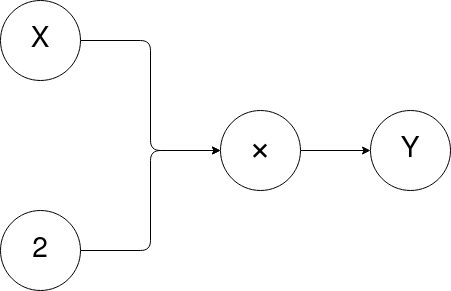
Figure-1: Computational graph for Y = X + 2

This is due to the ace of the gradient calculation. The gradients are required for optimization of the model weights. This computation graphs used for computing the gradients based on the chain rule and Jacobian matrix method. The gradient calculation can be automatically done using the backward function. If you want to compute the gradient of a tensor, you have to set the require_gradients parameter to true while defining the tensor.

x = torch.tensor([1,2,3,4])
w = torch.randn(1, require_gradients=True)
y = (x*y).sum()

y.backward()

print(f"dy/dx: {y.grad()}")
Python

4. Linear regression

Learning by doing a real project is a perfect way to gain some kinds of skills specially programming. To understand the basics of using the framework, it’s recommended to implement a simple mini project step by step from scratch. We choose linear regression as the training example and will go through the implementations from scratch and with out using pytorch. Then we will convert the code into using PyTorch and advanced functions.

4.1 Problem statement

Simple linear regression is used to estimate the relationship between two quantitative variables. You can use simple linear regression when you want to know:

How strong the relationship is between two variables (e.g., the relationship between rainfall and soil erosion).
The value of the dependent variable at a certain value of the independent variable (e.g., the amount of soil erosion at a certain level of rainfall).

Regression models describe the relationship between variables by fitting a line to the observed data. Linear regression models use a straight line, while logistic and nonlinear regression models use a curved line. Regression allows you to estimate how a dependent variable changes as the independent variable(s) change.

The formula for a simple linear regression is:

$y = \beta_{0} + \beta_{1} . X + \epsilon$

$y$ is the predicted value of the dependent variable ( $y$ ) for any given value of the independent variable ( $x$ ).
$\beta_0$ is the intercept, the predicted value of $y$ when the $x$ is $0$ .
$\beta_1$ is the regression coefficient – how much we expect $y$ to change as $x$ increases.
$x$ is the independent variable ( the variable we expect is influencing $y$ ).
$\epsilon$ is the error of the estimate, or how much variation there is in our estimate of the regression coefficient.

Linear regression finds the line of best fit line through your data by searching for the regression coefficient (B1) that minimizes the total error (e) of the model.

The loss function or error function in linear regression is determined by Mean Squared Error or MSE.

$L = \frac{1}{N} \sum_{i=1}^{N} (\hat{Y}_{i} - Y_{i})^2$

To minimize the error, we have to update the regression coefficients by computing the gradient with respect to the dependent variables (Model weights). And update the regression coefficients as below:

$w = w - \alpha.\frac{dJ}{dw}$

Which:

$\frac{dJ}{dw} = \frac{1}{N} . 2x . (\hat{y}-y)$

For this example we define a simple training set which is a set of 2D points $(x,y)$ such that $y = 2 \times x$ .

x	y
1	2
2	4
3	6
4	8
5	10
6	12

We pick $x=6$ as the test point and the rest as training data. Here is the implementation:

import numpy as np

# Training Data
X = np.array([1,2,3,4,5], dtype=np.float32)
Y = np.array([2,4,6,8,10], dtype=np.float32)

# Test Data
x_test = np.array([6], dtype=np.float32)
y_test = np.array([12], dtype=np.float32)
Python

The network will have a single node that has a single parameter $w$ which is randomly evaluated.

# Weights: A single node (no bias is considered)
w = np.random.rand()
Python

In PyTorch the forward pass in calculating the layer output is done by calling the forward function which, represents the forward pass of the network. In conclusion, we will call the model output function, the forward function.

# Forward pass:
# Predict the output of the network on the input data.
def forward(x, weights):
    return x*weights
Python

Then we have to define the loss function of the network which is the MSE loss function:

# Model loss function:
# MSE = 1/N * sum((y_i - y_hat_i)^2)
def mse(y,y_pred):
    return np.mean(np.square(y-y_pred))

print (f'prediction before training f({x_test}): {forward(x_test, weights)}')    
Python

Finally, we will need a function to calculate the gradient of the network coefficients, which in pytorch is called the backward function.

# Calculating gradients: 
# dJ/dw = 1/N * 2x *(w*x-y) // w*x = y_pred
def backward(x, y, w):
    return np.dot(2*x, (w*x-y)).mean()
Python

Finally, here is the training loop:

learning_rate = 0.01 # Alpha
num_epochs = 100

for epoch in range(num_epochs):
    # Forward pass: Compute predicted y by passing x to the model
    Y_pred = forward(X, w)

    # Compute and print loss
    loss = mse(Y, Y_pred)

    # Backward pass: Compute gradient of the loss with respect to model parameters
    dw = backward(X,Y,w)

    # Update parameters
    w = w - learning_rate * dw
    if (epoch) % 10 == 0:
        print(f"Epoch: {epoch} loss={loss:0.3f}, weights={[w]}")
        
print (f"Model prediction for x=6 is: {forward(x_test, weights):.3f})

Python

Epoch: 0 loss=24.130, weights=[2.14810945503594]
Epoch: 10 loss=0.000, weights=[2.0000000976789147]
Epoch: 20 loss=0.000, weights=[2.0000000976789147]
Epoch: 30 loss=0.000, weights=[2.0000000976789147]
Epoch: 40 loss=0.000, weights=[2.0000000976789147]
Epoch: 50 loss=0.000, weights=[2.0000000976789147]
Epoch: 60 loss=0.000, weights=[2.0000000976789147]
Epoch: 70 loss=0.000, weights=[2.0000000976789147]
Epoch: 80 loss=0.000, weights=[2.0000000976789147]
Epoch: 90 loss=0.000, weights=[2.0000000976789147]
Model prediction for x=6 is: [12.]

As you can see, the model converged after 100 iterations and successfully predicted the expected value for $x=6$ which is $y=12$ .

4.2 Including PyTorch

We implemented a simple linear regression model from scratch and only using numpy. Now it’s time to include PyTorch in our code. First, we have to turn every variable ( $x$ , $y$ and $w$ ) into a tensor instead of numpy arrays.

import torch

# Training Data
X = torch.tensor([1,2,3,4,5], dtype=torch.float32)
Y = torch.tensor([2,4,6,8,10], dtype=torch.float32)

# Test Data
x_test = torch.tensor([6], dtype=torch.float32)
y_test = torch.tensor([12], dtype=torch.float32)

# Weights: A single nuron
w = torch.randn(1, requires_grad=True, dtype=torch.float32)
Python

In the above code, while defining the weight parameter, we said that it requires tracking the gradient calculation for this tensor by setting the require_grad parameter to True. If we don’t set this parameter to True, while calling the backward function, it will throw an exception because it doesn’t store the gradients in the computation graph. So, be careful when defining a tensor which is required to calculate the gradients.

Next, we have to define the forward and loss function for the model.

# Forward pass:
# Predict the output of the network on the input data.
def forward(x, weights):
    return x*weights

# Model loss function:
# MSE = 1/N * sum((y_i - y_hat_i)^2)
def mse(y,y_pred):
    return ((y-y_pred)**2).mean()
Python

As we said in the previous section, gradients can be calculated by calling the backward function. For this reason, there is no need to define the backward function. While calling the backward function, the calculated gradients will remain in the computation graph until you free its memory. and this could be done by calling tensor.grad.zero_() function. So, be careful while calling the backward function and make sure that you free the memory associated with the gradients (you can see this in the code below).

Here is the training loop:

learning_rate = 0.01
num_epochs = 100

for epoch in range(num_epochs):
    y_pred = forward(X, weights)
    loss = mse(Y, y_pred)
    loss.backward()
    with torch.no_grad():
        w -= learning_rate * w.grad
    # You have to zero the gradients before calling the backward function in the next step
    w.grad.zero_()
    
    if (epoch) % 10 == 0:
        print(f"Epoch: {epoch} loss={loss:0.3f}, weights={w}")
        
print (f"Model prediction for x=6 is: {forward(x_test, w):.3f})
Python

Epoch: 0 loss=49.172, weights=tensor([0.9472], requires_grad=True)
Epoch: 10 loss=0.139, weights=tensor([1.9122], requires_grad=True)
Epoch: 20 loss=0.001, weights=tensor([1.9927], requires_grad=True)
Epoch: 30 loss=0.000, weights=tensor([1.9994], requires_grad=True)
Epoch: 40 loss=0.000, weights=tensor([1.9999], requires_grad=True)
Epoch: 50 loss=0.000, weights=tensor([2.0000], requires_grad=True)
Epoch: 60 loss=0.000, weights=tensor([2.0000], requires_grad=True)
Epoch: 70 loss=0.000, weights=tensor([2.0000], requires_grad=True)
Epoch: 80 loss=0.000, weights=tensor([2.0000], requires_grad=True)
Epoch: 90 loss=0.000, weights=tensor([2.0000], requires_grad=True)
Model prediction for x=6 is: tensor([12.0000], grad_fn=<MulBackward0>)

4.3 More including PyTorch

Now, let’s use the built-in PyTorch optimizer and loss function as well as the built-in forward function. First change that we should make is to remove the loss function that we where using and use the built-in MSELoss instead. Then, instead of manually updating the model parameters, we can use the built-in optimizers such as Stochastic Gradient Descent (SGD), Adam or etc.

As we know, this model is a single linear nuron which can be represented by torch.nn.linear(input_size, output_size). This layer has its own parameters which means it’s not required to define the weights parameter $w$ any more.

While using optimizers, calling optimizer.step() will automatically update the model parameters and optimizer.zero_grad() will automatically free the gradients memory.

import torch

# Training Data
X = torch.tensor([[1],[2],[3],[4],[5]], dtype=torch.float32)
Y = torch.tensor([[2],[4],[6],[8],[10]], dtype=torch.float32)

# Test Data
x_test = torch.tensor([6], dtype=torch.float32)
y_test = torch.tensor([12], dtype=torch.float32)

n_samples, n_features = X.shape

input_size = n_features
output_size = n_features

model = torch.nn.Linear(input_size, output_size)

print (f'prediction before training f({x_test}): {model(x_test).item():.3f}')    

learning_rate = 0.01
num_epochs = 2000

# using built-in SGD optimizer
optimizer = torch.optim.SGD(model.parameters(), lr=learning_rate)
# using built-in MSE loss function
loss = torch.nn.MSELoss()

for epoch in range(num_epochs):
    y_pred = model(X)
    l = loss(Y, y_pred)
    l.backward()
    optimizer.step()
    optimizer.zero_grad()
    
    if (epoch) % 500 == 0:
        print(f"Epoch: {epoch} loss={l.item():0.5f}, weights={weights[0].item():0.5f}")

print (f"{model(x_test).item():0.3f}") 
Python

prediction before training f(tensor([6.])): 0.314
Epoch: 0 loss=45.60832, weights=0.29675
Epoch: 500 loss=0.00051, weights=0.29675
Epoch: 1000 loss=0.00002, weights=0.29675
Epoch: 1500 loss=0.00000, weights=0.29675
12.000

4.4 Turning model into a Torch module

We can define blocks of layers as modules in PyTorch which are called modules. To do so, we have to define a class which inherits from the base torch.nn.Module class and implement the forward function for that module.

class Model(torch.nn.Module):
    
    def __init__(self):
        super(Model, self).__init__()
        self.ll_1 = torch.nn.Linear(1, 1)
        
    def forward(self, x):
        return self.ll_1(x)
Python

Now we can instantiate and use this model instead of defining a single fully connected layer as our model.

mport torch

# Training Data
X = torch.tensor([[1],[2],[3],[4],[5]], dtype=torch.float32)
Y = torch.tensor([[2],[4],[6],[8],[10]], dtype=torch.float32)

# Test Data
x_test = torch.tensor([6], dtype=torch.float32)
y_test = torch.tensor([12], dtype=torch.float32)

n_samples, n_features = X.shape

input_size = n_features
output_size = n_features

class Model(torch.nn.Module):
    
    def __init__(self, input_size, output_size):
        super(Model, self).__init__()
        self.ll_1 = torch.nn.Linear(input_size, output_size)
        
    def forward(self, x):
        return self.ll_1(x)

model = Model(input_size, output_size)

print (f'prediction before training f({x_test}): {model(x_test).item():.3f}')    

learning_rate = 0.01
num_epochs = 2000

# using built-in SGD optimizer
optimizer = torch.optim.SGD(model.parameters(), lr=learning_rate)
# using built-in MSE loss function
loss = torch.nn.MSELoss()

for epoch in range(num_epochs):
    y_pred = model(X)
    l = loss(Y, y_pred)
    l.backward()
    optimizer.step()
    optimizer.zero_grad()
    
    if (epoch) % 500 == 0:
        print(f"Epoch: {epoch} loss={l.item():0.5f}, weights={weights[0].item():0.5f}")

print (f"{model(x_test).item():0.3f}")
Python

4.5 More realistic example

Now lets use a more realistic data and plot the results with matplotlib.

import torch
from sklearn import datasets
import matplotlib.pyplot as plt
import numpy as np

dataset = datasets.make_regression(n_samples=20, n_features=1, noise=20, random_state=1)

X, Y = torch.from_numpy(dataset[0].astype(np.float32)), torch.from_numpy(dataset[1].astype(np.float32))
Y = Y.view(Y.shape[0], 1)
n_samples, n_features = X.shape

class Model(torch.nn.Module):
    def __init__(self):
        super(Model, self, input_size, output_size).__init__()
        self.ll_1 = torch.nn.Linear(1, 1)
        
    def forward(self, x):
        return self.ll_1(x)
    
    def parameters(self):
        return self.ll_1.parameters()

model = Model(n_features, n_features)

criterion = torch.nn.MSELoss()
optimizer = torch.optim.SGD(model.parameters(), lr=0.01)

num_epochs = 1000

for epoch in range(num_epochs):
    y_pred = model(X)
    loss = criterion(y_pred, Y)
    loss.backward()
    optimizer.step()
    optimizer.zero_grad()
    
    if (epoch+1) % 10 == 0:
        print(f'Epoch: {epoch+1}, Loss: {loss.item():.4f}')

prediction = model(X).detach().numpy()

plt.plot(X.detach().numpy(), Y.detach().numpy(), 'ro')
plt.plot(X.detach().numpy(), prediction, 'b')

Python

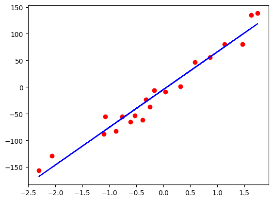
Figure-2: Regression results

5. Logistic regression

Here is a classification example using the breast cancer dataset from scikit-learn library. To recap, the problem statement is, we want to classify patients into two classes, having and not having the breast cancer using a single nuron as the previous examples.

import torch
import sklearn
import matplotlib.pyplot as plt
import numpy as np
from sklearn.model_selection import train_test_split

dataset = sklearn.datasets.load_breast_cancer()
X, y = dataset.data, dataset.target

n_samples, n_features = X.shape

x_train, x_test, y_train, y_test = train_test_split(X, y, test_size=0.2, random_state=42)

scaler = sklearn.preprocessing.StandardScaler()

x_train = scaler.fit_transform(x_train)
x_test = scaler.transform(x_test)

x_train = torch.from_numpy(x_train.astype(np.float32))
x_test = torch.from_numpy(x_test.astype(np.float32))

y_train = torch.from_numpy(y_train.astype(np.float32))
y_test = torch.from_numpy(y_test.astype(np.float32))

y_train = y_train.view(y_train.shape[0], 1)
y_test = y_test.view(y_test.shape[0], 1)

class LogisticRegression(torch.nn.Module):
    
    def __init__(self, num_features):
        super(LogisticRegression, self).__init__()
        self.linear = torch.nn.Linear(num_features, 1)
        
    def forward(self, x):
        y_pred = torch.sigmoid(self.linear(x))
        return y_pred

model = LogisticRegression(n_features)

criterion = torch.nn.BCELoss()
optimizer = torch.optim.SGD(model.parameters(), lr=0.01)

for epoch in range(100):
    y_pred = model(x_train)
    loss = criterion(y_pred, y_train)
    loss.backward()
    optimizer.step()
    optimizer.zero_grad()
    if epoch % 10 == 0:
        # Prevent tracking gradients during the below calculation
        with torch.no_grad():
            prediction = model(x_test).round()
            accuracy = prediction.eq(y_test).sum().item() / len(y_test)
            print(f'epoch: {epoch}, loss: {loss.item():.03f}, accuracy: {accuracy:.03f}')    
Python

As you can see, in the code, when we want to compute the accuracy of the model, we dont need to to keep track of calculated gradients of the calculation. To prevent this to affect our training and calculations, we have to turn this tracking off. This can be done by calling torch.no_grad() in a with block or making a detached copy of the variables directly by calling the tensor.detach() function of that tensor which returns a detached copy of that tensor and work with the returned value instead of the main tensor.

a = torch.tensor([1,2,3])
a_copy = a.detach()
# now use a_copy to compute the accuracy...
Python

epoch: 0, loss: 0.892, accuracy: 0.281
epoch: 10, loss: 0.650, accuracy: 0.667
epoch: 20, loss: 0.515, accuracy: 0.860
epoch: 30, loss: 0.433, accuracy: 0.939
epoch: 40, loss: 0.380, accuracy: 0.947
epoch: 50, loss: 0.342, accuracy: 0.965
epoch: 60, loss: 0.315, accuracy: 0.965
epoch: 70, loss: 0.293, accuracy: 0.965
epoch: 80, loss: 0.276, accuracy: 0.965
epoch: 90, loss: 0.262, accuracy: 0.965

6. Conclusion

In this section we learned what is PyTorch, Tensors and the computation graph definition. Then, we implemented a simple linear regression from scratch using numpy which helped us to better understanding the problem and how to solve the problem by implementation. After that, we turned the calculations from numpy into PyTorch tensors. Finally, we completed the implementation using built-in PyTorch optimizers and loss functions and some examples.