
This is a zero-to-one tutorial: it doesn’t assume you’ve used a deep learning framework before, only that you’re comfortable reading Python. By the end of this part you’ll understand what a tensor and a gradient actually are (not just how to type them), and you’ll have trained two real models — a linear regressor and a logistic-regression classifier — first from scratch with plain arithmetic, then rebuilt the same models in PyTorch piece by piece, so you can see exactly what the framework is doing for you at each step.
1. What are we actually doing?
Before any code: a “model” in machine learning is just a function with some adjustable numbers in it, called parameters or weights. Training a model means searching for values of those numbers that make the function’s output match reality as closely as possible, on examples you already know the answer to. Three ingredients make that search possible:
- Data — input/output pairs you already know are correct (e.g., “this house is 80m² and sold for $200k”).
- A loss function — a single number that says how wrong the model’s current output is compared to the real answer. Bigger loss, worse model.
- An optimization procedure — a way to nudge every weight slightly in the direction that would have made the loss smaller. Do this enough times, on enough examples, and the weights converge to something useful.
That third ingredient is where PyTorch earns its keep. Computing “which direction would have made the loss smaller” for every weight in a large model, by hand, is exactly the kind of calculus that gets unmanageable past a few parameters. PyTorch’s whole value proposition, distilled: it does that calculus for you automatically, and it does the (very repetitive) arithmetic on those weights fast, in parallel, ideally on a GPU. Everything in this post is really about those two things — automatic differentiation, and fast parallel arithmetic — with a specific framework’s syntax wrapped around them.
2. What is PyTorch, actually

PyTorch is an open-source library for exactly the two things above: tensor computation with strong GPU acceleration, and automatic differentiation over arbitrary Python code. It was originally developed at Facebook AI Research (FAIR) and first released publicly in 2016 [1]; the design and engineering behind it were formally written up in Paszke et al.’s 2019 NeurIPS paper, which is still the right reference if you want the “why it’s built this way” story from the people who built it [1]. In September 2022, Meta transferred PyTorch’s governance to the independent, vendor-neutral PyTorch Foundation under the Linux Foundation, with AMD, AWS, Google Cloud, Meta, Microsoft Azure, and NVIDIA as founding members [2] — so today it isn’t a single company’s internal tool, it’s genuinely community-governed infrastructure.
Two design choices explain most of what makes it pleasant to use, and both are worth naming because they’re the actual reasons researchers reach for it over the alternatives:
- Eager, define-by-run execution. Older frameworks (TensorFlow 1.x, Theano) made you build a static computation graph first and run data through it afterward — closer to writing a program that writes a program. PyTorch runs your Python code line by line, immediately, the same way any other Python code does; the “graph” gets built implicitly as a side effect of running your code, not as a separate step you author. This makes debugging trivial — you can drop a
print()or a debugger breakpoint anywhere, mid-model, and just look at real tensor values, because there’s no separate compiled graph hiding them from you. - Reverse-mode automatic differentiation via a dynamic tape, a design PyTorch adopted from the Chainer framework’s “define-by-run” approach [3]. Every operation on a tensor that’s tracking gradients gets recorded, in order, as it actually executes; running that tape backward afterward computes every gradient in one pass, using the chain rule. Because it’s the actual executed operations being recorded (not a pre-declared static graph), the graph can be different on every single call — which matters for models whose structure depends on the input (variable-length sequences, tree-structured data, control flow).
Beyond that, it’s simply a mature, actively maintained, Python-native project with excellent GPU support — which is most of why it’s become the default in ML research and a large share of production systems.
3. Installing PyTorch
You can follow this tutorial using an online platform such as Google Colab or Kaggle, which give you a Python environment through a Jupyter notebook and a proper GPU, more than enough for learning and even small projects or homework — both come with PyTorch already installed, so if you’re just starting out, this is genuinely the path of least resistance and you can skip straight to Section 4. If you want PyTorch on your own machine, here’s how.
3.1 Installing PyTorch locally
The official installer selector at pytorch.org [4] always has the current, correct command for your OS and CUDA version — treat it as the source of truth over any command frozen in a blog post, including this one, since exact package versions and CUDA compatibility shift over time.
If you haven’t installed Anaconda on your machine, download and install it, then create a dedicated environment (isolating dependencies per project like this avoids a huge and common class of “it works on my other project but not this one” bugs):
$ conda create --name torch python=3.9
After creating the environment, activate it:
$ conda activate torch
Then use pip to install PyTorch. If your machine has an NVIDIA GPU and you want CUDA acceleration, use the command the installer selector gives you for your CUDA version; if you don’t have a GPU, or just want the simplest possible install to follow along with this tutorial, the CPU-only build works identically for everything here, just slower on larger models:
$ pip install torch torchvision torchaudio
It will take some time, but it will install PyTorch and, if applicable, its GPU requirements on your machine.
To check whether GPU acceleration is actually available in your install, open a Python file and run:
import torch
print(f"Is GPU supported? {'Yes' if torch.cuda.is_available() else 'No'}")
Is GPU supported? Yes
Getting No here isn’t a failure — it just means everything below will run on CPU, which is perfectly fine for tensors and models this small. Well done, you have PyTorch installed and you’re ready to go through this tutorial.
4. Tensor basics
The most basic class in the PyTorch library is the tensor. Almost every variable and operation in PyTorch is represented by a tensor — think of it as PyTorch’s version of a NumPy array (a Python list generalizes to one dimension; a tensor generalizes to any number of them: a scalar is a 0-dimensional tensor, a vector is 1-D, a matrix is 2-D, a batch of RGB images is 4-D, and so on). The reason this specific abstraction exists, rather than just using Python lists, is that machine learning is fundamentally linear algebra — dot products, matrix multiplications, sums over large arrays — and a tensor library is what makes that fast: operations run as compiled, vectorized code (in C++/CUDA under the hood) instead of a slow Python for loop, and the exact same tensor can live on a CPU or be moved to a GPU to run in parallel across thousands of cores.
import torch

# Creating tensors
sample_tensor = torch.tensor([2, 2])
random_tensor = torch.randn(2, 2)   # random values, standard normal distribution
zero_tensor   = torch.zeros(2, 2)
one_tensor    = torch.ones(2, 2)
A few operations you’ll reach for constantly:
t = torch.tensor([[1, 2, 3], [4, 5, 6]])

t.shape          # torch.Size([2, 3]) — dimensions, the single most useful thing to check when debugging
t[0]              # tensor([1, 2, 3])  — indexing works like NumPy/Python lists
t[:, 1]           # tensor([2, 5])     — slicing: every row, column 1
t.sum()           # tensor(21)
t.mean()          # only works on float tensors — int tensors will raise an error here
t + 10            # tensor([[11, 12, 13], [14, 15, 16]]) — elementwise, "broadcast" over every element
t.item()          # only valid on a single-element tensor; pulls out a plain Python number
That last one, .item(), trips people up early on: a tensor is not a Python number, even a 0-dimensional one holding a single value — you’ll see it throughout this tutorial whenever we need to print a loss as an ordinary float.
You can reshape a tensor with .view(), which behaves like NumPy’s reshape (with one catch: .view() requires the underlying memory to be contiguous, which is the usual case for tensors you just created, but can bite you after certain operations like .transpose() — if you ever hit a RuntimeError about a view needing contiguous memory, calling .reshape() instead, or .contiguous() first, is the fix):
sample_tensor = torch.tensor([[1,  2,   3,   4 ],
                              [5,  6,   7,   8 ],
                              [9,  10,  11,  12],
                              [13, 14,  15,  16]])

# turn into a 1-D tensor ([1, 2, 3, ..., 16])
one_dimension_tensor = sample_tensor.view(16, 1)
Tensors interoperate with NumPy directly and cheaply — torch.from_numpy(array) wraps a NumPy array as a tensor without copying its data, and tensor.numpy() goes the other way — which is why you’ll see both libraries mixed freely in the same script; most datasets get loaded and preprocessed with NumPy/pandas/scikit-learn, then handed to PyTorch at the model boundary.
Tensors can live on the CPU or the GPU, and math between two tensors requires both to be on the same device — a very common beginner error is a RuntimeError about tensors on different devices, usually because one tensor got moved to the GPU and another didn’t. Move a tensor with .to(...):
device = torch.device('cuda' if torch.cuda.is_available() else 'cpu')

sample_tensor = torch.tensor([2, 2])
sample_tensor = sample_tensor.to(device)   # now lives on `device`
Writing device once like that, driven by torch.cuda.is_available(), and reusing it everywhere, is the standard pattern for code that should run unmodified whether or not a GPU is present — you’ll see it throughout the rest of this series.
4.1 Operations and gradient calculation
Every calculation you run on tensors that have gradient-tracking turned on gets recorded by PyTorch as a computation graph — a record of exactly which operations produced which values, in order. Take a tiny example: y = (x * w).sum(). As Python executes that line, PyTorch is quietly building this graph behind the scenes:
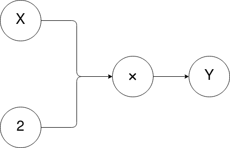
Figure 1: computation graph for a multiply followed by a sum
That graph is what makes automatic gradient calculation possible: to know how much the final output y would change if we nudged w slightly, PyTorch walks this graph backward, from y to w, applying the chain rule at every step it passes through — exactly the calculus you’d do by hand for a small expression like this one, just done automatically and for expressions with millions of operations. This one calculation — “how sensitive is the loss to each weight” — is the gradient, and it’s the single quantity every training loop in this post exists to compute and then act on.
To make a tensor participate in this recording, set requires_grad=True when you create it (only tensors you’ll be optimizing — your model’s weights — normally need this; your input data doesn’t). Once you’ve computed a final scalar value (like a loss), calling .backward() on it walks the whole graph backward and populates .grad on every tensor that required gradients:
x = torch.tensor([1., 2., 3., 4.])
w = torch.randn(1, requires_grad=True)
y = (x * w).sum()

y.backward()

print(f"dy/dw: {w.grad}")
A couple of things worth knowing before you hit them as confusing errors later: calling .backward() on anything that isn’t a single scalar will raise an error unless you pass it an explicit gradient argument, because “the gradient of a vector with respect to another vector” isn’t a single well-defined thing the way it is for a scalar loss — this is part of why every loss function you’ll see in this post reduces its output to one number (with .mean() or .sum()) before anything gets trained on it. And gradients accumulate by default — calling .backward() twice adds the new gradients on top of the old ones rather than replacing them, which is exactly why every training loop later in this post explicitly zeroes gradients out before each new backward pass; forgetting that line is one of the most common silent bugs in PyTorch code (the model still trains, just wrong, since gradients from old steps keep leaking into new ones).
If you want to build this exact mechanism yourself, by hand, in about 150 lines of Python — genuinely worth doing once, to fully de-mystify what .backward() is doing — Andrej Karpathy’s micrograd walkthrough builds a tiny autograd engine from scratch and is the best beginner-level treatment of this I know of [5].
5. Linear regression
Learning by doing a real project is the fastest way to build intuition, especially with a new framework. We’ll implement linear regression three times, each version building on the last: from scratch with plain NumPy (no PyTorch at all, so you see exactly what’s being computed), then converted to PyTorch tensors with manual gradient updates (so you see exactly what .backward() replaces), then finally using PyTorch’s built-in optimizer, loss function, and layer classes (so you see what you actually write day to day). Linear regression is also, not coincidentally, the smallest possible neural network — a single neuron, with one weight and no activation function — so everything you learn about training it generalizes directly to bigger networks later in this series.
5.1 Problem statement
Simple linear regression estimates the relationship between two quantitative variables by fitting a straight line through observed data. It answers questions like:
- How strong is the relationship between two variables? (e.g., rainfall and soil erosion)
- What value would the dependent variable take at a given value of the independent variable? (e.g., expected erosion at a specific rainfall level)
The formula for simple linear regression:
\[y = \beta_{0} + \beta_{1} \cdot X + \epsilon\]- \(y\) is the predicted value of the dependent variable for a given \(x\).
- \(\beta_0\) is the intercept — the predicted \(y\) when \(x = 0\).
- \(\beta_1\) is the regression coefficient — how much \(y\) changes as \(x\) increases by 1.
- \(x\) is the independent variable.
- \(\epsilon\) is the error — the gap between the line’s prediction and the real data.
Linear regression finds the line of best fit by searching for the coefficient \(\beta_1\) that minimizes total error. That “total error” is measured by a loss function — here, Mean Squared Error (MSE), which squares each prediction’s error (so positive and negative errors don’t cancel out, and big misses are punished disproportionately more than small ones) and averages over all examples:
\[L = \frac{1}{N} \sum_{i=1}^{N} (\hat{Y}_{i} - Y_{i})^2\]To minimize that loss, we repeatedly nudge the weight in the direction that reduces it — this is gradient descent, and it’s the “optimization procedure” from Section 1 made concrete:
\[w = w - \alpha \cdot \frac{dJ}{dw}\]Here \(\alpha\) (alpha) is the learning rate — how big a step to take on each update. Too small, and training crawls; too large, and updates can overshoot and diverge instead of converging (worth remembering: if a training loop’s loss explodes to NaN or grows instead of shrinking, an oversized learning rate is the first thing to suspect). \(\frac{dJ}{dw}\) — the gradient — is exactly the quantity from Section 4.1 that tells us which direction reduces the loss, and for this specific loss and model it works out to:
You won’t need to derive that formula yourself once PyTorch is doing the differentiation — but seeing it once, and then implementing it by hand below, is exactly what makes .backward() feel like less of a black box.
For this example we’ll use a deliberately trivial training set — 2D points \((x, y)\) where \(y = 2 \times x\) — specifically because the right answer (\(w=2\)) is obvious, so it’s easy to tell at a glance whether training actually worked:
| x | y |
|---|---|
| 1 | 2 |
| 2 | 4 |
| 3 | 6 |
| 4 | 8 |
| 5 | 10 |
| 6 | 12 |
We’ll hold out \(x=6\) as a test point the model never trains on, and use the rest as training data:
import numpy as np

# Training Data
X = np.array([1,2,3,4,5], dtype=np.float32)
Y = np.array([2,4,6,8,10], dtype=np.float32)

# Test Data
x_test = np.array([6], dtype=np.float32)
y_test = np.array([12], dtype=np.float32)
The network will have a single node with a single parameter \(w\), initialized to a random value (training’s whole job is to move this random guess toward the correct one):
# Weights: a single node (no bias for now)
w = np.random.rand()
We’ll structure this from-scratch implementation the same way PyTorch structures its own models: with a forward function that computes the network’s output from its input and weights. It’s a small bit of extra ceremony here, but it means the switch to actual PyTorch in Section 5.2 will feel completely familiar.
# Forward pass:
# Predict the output of the network on the input data.
def forward(x, weights):
    return x * weights
Then the loss function — MSE, as derived above:
# Model loss function:
# MSE = 1/N * sum((y_i - y_hat_i)^2)
def mse(y, y_pred):
    return np.mean(np.square(y - y_pred))

print(f'prediction before training f({x_test}): {forward(x_test, w)}')
And a function to compute the gradient — in PyTorch, this entire function is what .backward() replaces:
# Calculating gradients:
# dJ/dw = 1/N * 2x * (w*x - y)   // note: w*x is y_pred
def backward(x, y, w):
    return np.dot(2*x, (w*x - y)).mean()
And finally, the training loop — this exact shape (forward pass, compute loss, backward pass, update weights, repeat) is the shape of every training loop you’ll write, in this post and beyond:
learning_rate = 0.01  # alpha
num_epochs = 100       # one epoch = one full pass over the training data

for epoch in range(num_epochs):
    # Forward pass: compute predicted y by passing x through the model
    Y_pred = forward(X, w)

    # Compute the loss, just to track/print it
    loss = mse(Y, Y_pred)

    # Backward pass: compute the gradient of the loss w.r.t. the model's weight
    dw = backward(X, Y, w)

    # Update the weight
    w = w - learning_rate * dw
    if epoch % 10 == 0:
        print(f"Epoch: {epoch} loss={loss:0.3f}, weights={[w]}")

print(f"Model prediction for x=6 is: {forward(x_test, w)}")
Epoch: 0 loss=24.130, weights=[2.14810945503594]
Epoch: 10 loss=0.000, weights=[2.0000000976789147]
Epoch: 20 loss=0.000, weights=[2.0000000976789147]
Epoch: 30 loss=0.000, weights=[2.0000000976789147]
Epoch: 40 loss=0.000, weights=[2.0000000976789147]
Epoch: 50 loss=0.000, weights=[2.0000000976789147]
Epoch: 60 loss=0.000, weights=[2.0000000976789147]
Epoch: 70 loss=0.000, weights=[2.0000000976789147]
Epoch: 80 loss=0.000, weights=[2.0000000976789147]
Epoch: 90 loss=0.000, weights=[2.0000000976789147]
Model prediction for x=6 is: [12.]
The model converged well before 100 iterations and correctly predicted \(y=12\) for the held-out \(x=6\) — not because it memorized that pair (it never saw it during training), but because it learned the actual underlying rule, \(y = 2x\).
5.2 Including PyTorch
Now let’s bring PyTorch in, one piece at a time. First, every variable (\(x\), \(y\), \(w\)) becomes a tensor instead of a NumPy array:
import torch

# Training Data
X = torch.tensor([1,2,3,4,5], dtype=torch.float32)
Y = torch.tensor([2,4,6,8,10], dtype=torch.float32)

# Test Data
x_test = torch.tensor([6], dtype=torch.float32)
y_test = torch.tensor([12], dtype=torch.float32)

# Weights: a single neuron
w = torch.randn(1, requires_grad=True, dtype=torch.float32)
Notice requires_grad=True on w specifically — per Section 4.1, that’s what tells PyTorch to track this tensor’s operations for differentiation. X and Y don’t need it; we’re never going to compute a gradient with respect to the data, only with respect to the weight. Forgetting requires_grad=True here is a common early mistake — calling .backward() later will raise an error, because the tensor was never recorded onto the computation graph in the first place.
Forward pass and loss function, unchanged in spirit from the NumPy version, just written with tensor operations:
# Forward pass:
# Predict the output of the network on the input data.
def forward(x, weights):
    return x * weights

# Model loss function:
# MSE = 1/N * sum((y_i - y_hat_i)^2)
def mse(y, y_pred):
    return ((y - y_pred) ** 2).mean()
There’s no backward function to write this time — that’s the entire point. Calling .backward() on the loss computes every gradient PyTorch needs, and stores it on w.grad. Two details matter once you do this in a loop: gradients accumulate (per Section 4.1) so we must zero them each iteration with w.grad.zero_(), and the weight update itself must happen outside gradient tracking — wrapped in with torch.no_grad(): — because “subtract the gradient from the weight” is itself a tensor operation, and we don’t want that operation recorded onto the graph for next time.
learning_rate = 0.01
num_epochs = 100

for epoch in range(num_epochs):
    y_pred = forward(X, w)
    loss = mse(Y, y_pred)
    loss.backward()
    with torch.no_grad():
        w -= learning_rate * w.grad
    # zero the gradient before the next backward() call — see Section 4.1
    w.grad.zero_()

    if epoch % 10 == 0:
        print(f"Epoch: {epoch} loss={loss:0.3f}, weights={w}")

print(f"Model prediction for x=6 is: {forward(x_test, w)}")
Epoch: 0 loss=49.172, weights=tensor([0.9472], requires_grad=True)
Epoch: 10 loss=0.139, weights=tensor([1.9122], requires_grad=True)
Epoch: 20 loss=0.001, weights=tensor([1.9927], requires_grad=True)
Epoch: 30 loss=0.000, weights=tensor([1.9994], requires_grad=True)
Epoch: 40 loss=0.000, weights=tensor([1.9999], requires_grad=True)
Epoch: 50 loss=0.000, weights=tensor([2.0000], requires_grad=True)
Epoch: 60 loss=0.000, weights=tensor([2.0000], requires_grad=True)
Epoch: 70 loss=0.000, weights=tensor([2.0000], requires_grad=True)
Epoch: 80 loss=0.000, weights=tensor([2.0000], requires_grad=True)
Epoch: 90 loss=0.000, weights=tensor([2.0000], requires_grad=True)
Model prediction for x=6 is: tensor([12.0000], grad_fn=<MulBackward0>)
Same result as the NumPy version, but the gradient was never derived or coded by hand — loss.backward() did section 5.1’s backward() function for us, automatically, for whatever loss function we’d written.
5.3 Using PyTorch’s built-in layers and optimizer
Manually subtracting learning_rate * w.grad is itself boilerplate PyTorch can take over. Instead of hand-updating weights, we use an optimizer — Stochastic Gradient Descent (SGD) here, though PyTorch ships several (Adam being the other one you’ll see constantly). And instead of a bare weight w, we use a built-in layer, torch.nn.Linear(input_size, output_size), which is precisely a single linear neuron like ours — it creates and owns its own weight (and, by default, a bias term \(\beta_0\)) internally, so we no longer define w ourselves at all.
import torch

# Training Data — note the shape: PyTorch's nn.Linear expects each
# sample as its own row, so a "5 samples, 1 feature" tensor is 5x1, not flat.
X = torch.tensor([[1],[2],[3],[4],[5]], dtype=torch.float32)
Y = torch.tensor([[2],[4],[6],[8],[10]], dtype=torch.float32)

# Test Data
x_test = torch.tensor([6], dtype=torch.float32)
y_test = torch.tensor([12], dtype=torch.float32)

n_samples, n_features = X.shape

input_size = n_features   # 1 input value per sample
output_size = 1           # 1 output value per sample — we set this explicitly,
                           # rather than reusing n_features, because input and
                           # output size are conceptually independent; they only
                           # happen to both be 1 in this particular example.

model = torch.nn.Linear(input_size, output_size)

print(f'prediction before training f({x_test}): {model(x_test).item():.3f}')

learning_rate = 0.01
num_epochs = 2000

optimizer = torch.optim.SGD(model.parameters(), lr=learning_rate)
loss_fn = torch.nn.MSELoss()

for epoch in range(num_epochs):
    y_pred = model(X)
    # PyTorch loss functions take (prediction, target) — that order matters
    # for losses that aren't symmetric (MSE happens to not care, but get in
    # the habit now, because most losses do).
    loss = loss_fn(y_pred, Y)
    loss.backward()
    optimizer.step()       # applies every parameter's update, using its .grad
    optimizer.zero_grad()  # equivalent to calling .grad.zero_() on every parameter

    if epoch % 500 == 0:
        print(f"Epoch: {epoch} loss={loss.item():0.5f}, weight={model.weight.item():0.5f}")

print(f"{model(x_test).item():0.3f}")
prediction before training f(tensor([6.])): 0.314
Epoch: 0 loss=45.60832, weight=0.29675
Epoch: 500 loss=0.00051, weight=1.98523
Epoch: 1000 loss=0.00002, weight=1.99979
Epoch: 1500 loss=0.00000, weight=1.99999
12.000
optimizer.step() and optimizer.zero_grad() are doing exactly what section 5.2’s manual with torch.no_grad(): w -= learning_rate * w.grad and w.grad.zero_() did — just generalized to work over every parameter in a model automatically, which matters enormously once a model has thousands or millions of them and hand-updating each one individually stops being an option.
5.4 Wrapping the model in a Module
Real models are rarely a single nn.Linear call — they’re stacks of layers. PyTorch’s convention for this is a Module: a class inheriting from torch.nn.Module that owns some layers in __init__ and defines how data flows through them in forward.
class Model(torch.nn.Module):

    def __init__(self, input_size, output_size):
        super(Model, self).__init__()
        self.ll_1 = torch.nn.Linear(input_size, output_size)

    def forward(self, x):
        return self.ll_1(x)
torch.nn.Module is what makes model.parameters() (used above by the optimizer) automatically discover every weight in every layer you assign as an attribute in __init__ — you never register parameters by hand, the base class does it via a bit of Python attribute-assignment magic. Using this Model class is a drop-in replacement for the bare nn.Linear from Section 5.3:
model = Model(input_size, output_size)
optimizer = torch.optim.SGD(model.parameters(), lr=learning_rate)
loss_fn = torch.nn.MSELoss()

for epoch in range(num_epochs):
    y_pred = model(X)
    loss = loss_fn(y_pred, Y)
    loss.backward()
    optimizer.step()
    optimizer.zero_grad()

    if epoch % 500 == 0:
        print(f"Epoch: {epoch} loss={loss.item():0.5f}, weight={model.ll_1.weight.item():0.5f}")

print(f"{model(x_test).item():0.3f}")
This is the pattern practically every PyTorch model you’ll ever see follows, from a single linear layer up to a modern transformer: subclass nn.Module, declare layers in __init__, wire them together in forward.
5.5 A more realistic example
Our toy dataset was exactly linear on purpose, to make correctness obvious. Real data has noise. Let’s generate a noisy synthetic dataset with scikit-learn and plot the fitted line with matplotlib, to see the model doing something closer to real regression:
import torch
from sklearn import datasets
import matplotlib.pyplot as plt
import numpy as np

dataset = datasets.make_regression(n_samples=20, n_features=1, noise=20, random_state=1)

X, Y = torch.from_numpy(dataset[0].astype(np.float32)), torch.from_numpy(dataset[1].astype(np.float32))
Y = Y.view(Y.shape[0], 1)
n_samples, n_features = X.shape

class Model(torch.nn.Module):
    def __init__(self, input_size, output_size):
        super(Model, self).__init__()
        self.ll_1 = torch.nn.Linear(input_size, output_size)

    def forward(self, x):
        return self.ll_1(x)

model = Model(n_features, 1)

criterion = torch.nn.MSELoss()
optimizer = torch.optim.SGD(model.parameters(), lr=0.01)

num_epochs = 1000

for epoch in range(num_epochs):
    y_pred = model(X)
    loss = criterion(y_pred, Y)
    loss.backward()
    optimizer.step()
    optimizer.zero_grad()

    if (epoch+1) % 10 == 0:
        print(f'Epoch: {epoch+1}, Loss: {loss.item():.4f}')

# .detach() drops a tensor's gradient-tracking (per Section 4.1) so it can be
# safely handed to NumPy/matplotlib, which know nothing about autograd.
prediction = model(X).detach().numpy()

plt.plot(X.detach().numpy(), Y.detach().numpy(), 'ro')
plt.plot(X.detach().numpy(), prediction, 'b')
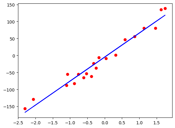
Figure 2: regression results — the fitted line (blue) through noisy data (red)
6. Logistic regression
Linear regression predicts a continuous number. Classification — predicting one of a fixed set of categories — needs a different output shape and a different loss, but reuses everything else we’ve built. Here’s a real classification example using the breast cancer dataset bundled with scikit-learn: predicting whether a tumor is malignant or benign from 30 measured features, using a single neuron, just like before.
Two changes from linear regression, both worth understanding rather than memorizing: a linear layer’s raw output can be any real number, but we want a probability (something between 0 and 1), so we pass it through the sigmoid function, which squashes any real number into that range; and for probabilities specifically, MSE is a poor loss (it doesn’t punish confidently-wrong predictions harshly enough), so we use Binary Cross-Entropy (BCE) loss instead, which does.
import torch
import matplotlib.pyplot as plt
import numpy as np
from sklearn.datasets import load_breast_cancer
from sklearn.model_selection import train_test_split
from sklearn.preprocessing import StandardScaler

dataset = load_breast_cancer()
X, y = dataset.data, dataset.target

n_samples, n_features = X.shape

x_train, x_test, y_train, y_test = train_test_split(X, y, test_size=0.2, random_state=42)

# Feature scaling matters here in a way it didn't for our toy example:
# the 30 features are on wildly different scales (e.g. "mean radius" vs.
# "mean area"), and gradient descent converges far more reliably when every
# feature is on a comparable scale. Fit the scaler on training data only,
# then apply the same transform to the test set — fitting on test data would
# leak information from the test set into training.
scaler = StandardScaler()
x_train = scaler.fit_transform(x_train)
x_test = scaler.transform(x_test)

x_train = torch.from_numpy(x_train.astype(np.float32))
x_test = torch.from_numpy(x_test.astype(np.float32))

y_train = torch.from_numpy(y_train.astype(np.float32))
y_test = torch.from_numpy(y_test.astype(np.float32))

y_train = y_train.view(y_train.shape[0], 1)
y_test = y_test.view(y_test.shape[0], 1)

class LogisticRegression(torch.nn.Module):

    def __init__(self, num_features):
        super(LogisticRegression, self).__init__()
        self.linear = torch.nn.Linear(num_features, 1)

    def forward(self, x):
        y_pred = torch.sigmoid(self.linear(x))
        return y_pred

model = LogisticRegression(n_features)

criterion = torch.nn.BCELoss()
optimizer = torch.optim.SGD(model.parameters(), lr=0.01)

for epoch in range(100):
    y_pred = model(x_train)
    loss = criterion(y_pred, y_train)
    loss.backward()
    optimizer.step()
    optimizer.zero_grad()
    if epoch % 10 == 0:
        # We don't need gradients for evaluation — only for training — so we
        # turn tracking off here, same idea as torch.no_grad() in Section 5.2.
        with torch.no_grad():
            prediction = model(x_test).round()
            accuracy = prediction.eq(y_test).sum().item() / len(y_test)
            print(f'epoch: {epoch}, loss: {loss.item():.03f}, accuracy: {accuracy:.03f}')
As in the training loop, when we only want to read a value (like accuracy) rather than train on it, we don’t need gradient tracking. torch.no_grad() turns it off for an entire block; the equivalent for a single tensor is .detach(), which returns a copy of the tensor that’s no longer connected to the computation graph:
a = torch.tensor([1, 2, 3], dtype=torch.float32, requires_grad=True)
a_copy = a.detach()  # same values, but detached from the graph
epoch: 0, loss: 0.892, accuracy: 0.281
epoch: 10, loss: 0.650, accuracy: 0.667
epoch: 20, loss: 0.515, accuracy: 0.860
epoch: 30, loss: 0.433, accuracy: 0.939
epoch: 40, loss: 0.380, accuracy: 0.947
epoch: 50, loss: 0.342, accuracy: 0.965
epoch: 60, loss: 0.315, accuracy: 0.965
epoch: 70, loss: 0.293, accuracy: 0.965
epoch: 80, loss: 0.276, accuracy: 0.965
epoch: 90, loss: 0.262, accuracy: 0.965
96.5% accuracy from a single neuron, no hidden layers at all — a reasonable reminder that a lot of real classification problems are closer to linear than intuition suggests.
7. Conclusion
Starting from “what does training even mean,” we built up to tensors, autograd, and the computation graph that makes .backward() possible; then implemented linear regression three times — from scratch, with manual PyTorch gradients, and with built-in optimizers and layers — so each abstraction had something concrete underneath it before we started trusting it; then reused every piece of that for a real logistic regression classifier. That five-line training loop (forward, loss, backward, step, zero_grad) is the actual core of this entire post, and it’s the same five lines whether the model has one parameter or one billion.
Part 2 picks up where the raw NumPy arrays in this post get replaced with something that scales: PyTorch’s Dataset and DataLoader, for when your data doesn’t fit conveniently in five lines of Python.
References
- A. Paszke, S. Gross, F. Massa, A. Lerer, et al. PyTorch: An Imperative Style, High-Performance Deep Learning Library. Advances in Neural Information Processing Systems 32 (NeurIPS 2019), pp. 8024–8035. papers.nips.cc
- Linux Foundation. Meta Transitions PyTorch to the Linux Foundation. September 2022. linuxfoundation.org
- S. Tokui, K. Oono, S. Hido, J. Clayton. Chainer: a Next-Generation Open Source Framework for Deep Learning. NeurIPS Workshop on Machine Learning Systems, 2015.
- PyTorch. Get Started: Locally. pytorch.org/get-started/locally
- A. Karpathy. The spelled-out intro to neural networks and backpropagation: building micrograd. Neural Networks: Zero to Hero. github.com/karpathy/micrograd · video
- PyTorch.
torch.Tensordocumentation. pytorch.org/docs/stable/tensors.html - PyTorch. Autograd mechanics. pytorch.org/docs/stable/notes/autograd.html
Comment Channel